Load the aggregated food groups and their attributes. We have 28 food groups.
<- read.csv ('data/foods.csv' , sep = ',' ):: setDT (foods) # use data.table format 1 : 10 ,] # show the first 10
                   food intake energy protein   fat carbs sugar alcohol  ghge
                 <char>  <num>  <num>   <num> <num> <num> <num>   <num> <num>
 1:               Bread  175.4 10.696   0.091 0.030 0.441 0.002       0 0.001
 2:        Other grains   45.0 14.022   0.100 0.042 0.607 0.011       0 0.002
 3:               Cakes   35.6 14.185   0.067 0.152 0.424 0.185       0 0.002
 4:            Potatoes   67.8  3.791   0.021 0.007 0.178 0.000       0 0.000
 5:          Vegetables  154.6  1.565   0.015 0.008 0.050 0.005       0 0.001
 6:             Legumes    3.5  8.571   0.143 0.029 0.286 0.000       0 0.001
 7:      Fruit, berries  171.5  2.729   0.008 0.004 0.134 0.029       0 0.001
 8:               Juice  111.0  1.928   0.005 0.002 0.103 0.000       0 0.001
 9:                Nuts    4.3 25.581   0.209 0.535 0.116 0.000       0 0.005
10: Vegetarian products    0.7  4.286   0.143 0.000 0.000 0.000       0 0.003
Define the constraints on
energy
protein, fat, carbs, sugar, alcohol
GHGE (greenhouse gas equivalent)
<- data.frame (constraint = c ('lower' , 'upper' ), energy = c (9000 , 10000 ), protein = c (55 , 111.5 ), fat = c (61.8 , 98.8 ), carbs = c (250 , 334.6 ), sugar = c (0 , 54.8 ), alcohol = c (0 , 10 ),ghge = c (0 , 4.7 )
  constraint energy protein  fat carbs sugar alcohol ghge
1      lower   9000    55.0 61.8 250.0   0.0       0  0.0
2      upper  10000   111.5 98.8 334.6  54.8      10  4.7
Exploratory data analysis on current diet
Before we construct the optimization problem, we should always understand the data. This helps us picking the important food groups, as well as making sense of the constraints.
# compute the contribution (indiv * intake) for 28 foods <- apply (X = foods[, c ('energy' , 'protein' , 'fat' , 'carbs' , 'sugar' , 'alcohol' , 'ghge' )], MARGIN = 2 , FUN = function (x){x* foods$ intake})rownames (ftotal) <- foods$ food # name the rows head (ftotal)
                energy protein    fat   carbs  sugar alcohol   ghge
Bread        1876.0784 15.9614 5.2620 77.3514 0.3508       0 0.1754
Other grains  630.9900  4.5000 1.8900 27.3150 0.4950       0 0.0900
Cakes         504.9860  2.3852 5.4112 15.0944 6.5860       0 0.0712
Potatoes      257.0298  1.4238 0.4746 12.0684 0.0000       0 0.0000
Vegetables    241.9490  2.3190 1.2368  7.7300 0.7730       0 0.1546
Legumes        29.9985  0.5005 0.1015  1.0010 0.0000       0 0.0035
We can also examine whether the current intake satisfy the constraints from above. For example, the energy contribution from bread is \(175.4 \times 10.696\) , which is the intake times per unit energy.
t (as.matrix (foods$ intake)) %*% as.matrix (foods[, .(energy, protein, fat, carbs, sugar, alcohol, ghge)])
       energy protein     fat    carbs   sugar alcohol   ghge
[1,] 9314.278 98.2159 85.7644 234.7172 39.2148  8.6498 3.7807
It looks like all categories but carbs fall within the expected range. Carb is slighter lower than the lower threshold.
Now we can compute the percentage of each one of the 28 food group contribution towards the total.
# divide by total of all 28 (upper constraints) <- apply (ftotal, 2 , sum)
   energy   protein       fat     carbs     sugar   alcohol      ghge
9314.2778   98.2159   85.7644  234.7172   39.2148    8.6498    3.7807
<- t (apply (X = ftotal, MARGIN = 1 , FUN = function (x){x/ fsum}))<- round (fprop, digits = 3 ) # keep 3 digits rownames (fprop) <- foods$ foodhead (fprop)
             energy protein   fat carbs sugar alcohol  ghge
Bread         0.201   0.163 0.061 0.330 0.009       0 0.046
Other grains  0.068   0.046 0.022 0.116 0.013       0 0.024
Cakes         0.054   0.024 0.063 0.064 0.168       0 0.019
Potatoes      0.028   0.014 0.006 0.051 0.000       0 0.000
Vegetables    0.026   0.024 0.014 0.033 0.020       0 0.041
Legumes       0.003   0.005 0.001 0.004 0.000       0 0.001
For example, bread contributes to 20% towards the total energy, and 16.3% of the total protein.
Visualization
In this section we are mostly focused on energy, intake, ghge . It is easy to extend to other macronutrient categories.
We need some more data manipulation before plotting.
Show code
# first define big groups <- c ('Bread' , 'Other grains' , 'Cakes' )<- c ('Potatoes' , 'Vegetables' , 'Legumes' , 'Fruit, berries' , 'Juice' , 'Nuts' , 'Vegetarian products' )<- c ('Red meat' , 'White meat' )<- c ('Fish' , 'Eggs' )<- c ('Cream, cream desserts' , 'Milk, yoghurt' , 'Cheese' )<- c ('Butter, margarine, oil' )<- c ('Coffee, tea' , 'Soda, saft' , 'Water' , 'Alcoholic beverages' , 'Non-dairy milk' )<- c ('Sugar, sweets' , 'Snacks' , 'Sauces' , 'Spices' , 'Other' )# reorder food names to make the plot easier to read <- c (grain, fruit_vege, meat, fish_egg,
 [1] "Bread"                  "Other grains"           "Cakes"
 [4] "Potatoes"               "Vegetables"             "Legumes"
 [7] "Fruit, berries"         "Juice"                  "Nuts"
[10] "Vegetarian products"    "Red meat"               "White meat"
[13] "Fish"                   "Eggs"                   "Cream, cream desserts"
[16] "Milk, yoghurt"          "Cheese"                 "Butter, margarine, oil"
[19] "Coffee, tea"            "Soda, saft"             "Water"
[22] "Alcoholic beverages"    "Non-dairy milk"         "Sugar, sweets"
[25] "Snacks"                 "Sauces"                 "Spices"
[28] "Other"
Show code
# require some data manip # need big food group, food name (smaller food group) <- data.frame (ftotal) # total $ food_name <- row.names (pdt)<- data.table:: setDT (pdt)# attach big group %in% grain, big_group : = 'grain' ]%in% fruit_vege, big_group : = 'fruit_vege' ]%in% meat, big_group : = 'meat' ]%in% fish_egg, big_group : = 'fish_egg' ]%in% dairy, big_group : = 'dairy' ]%in% fats, big_group : = 'fats' ]%in% beverages, big_group : = 'beverages' ]%in% sugar_other, big_group : = 'sugar_other' ]# make long format <- tidyr:: pivot_longer (pdt, cols = - c (food_name, big_group),names_to = 'category' )<- data.table:: setDT (pdt_long)# new variable, food_name_order $ food_name_order <- factor (pdt_long$ food_name, levels = names_ordered, labels = names_ordered)
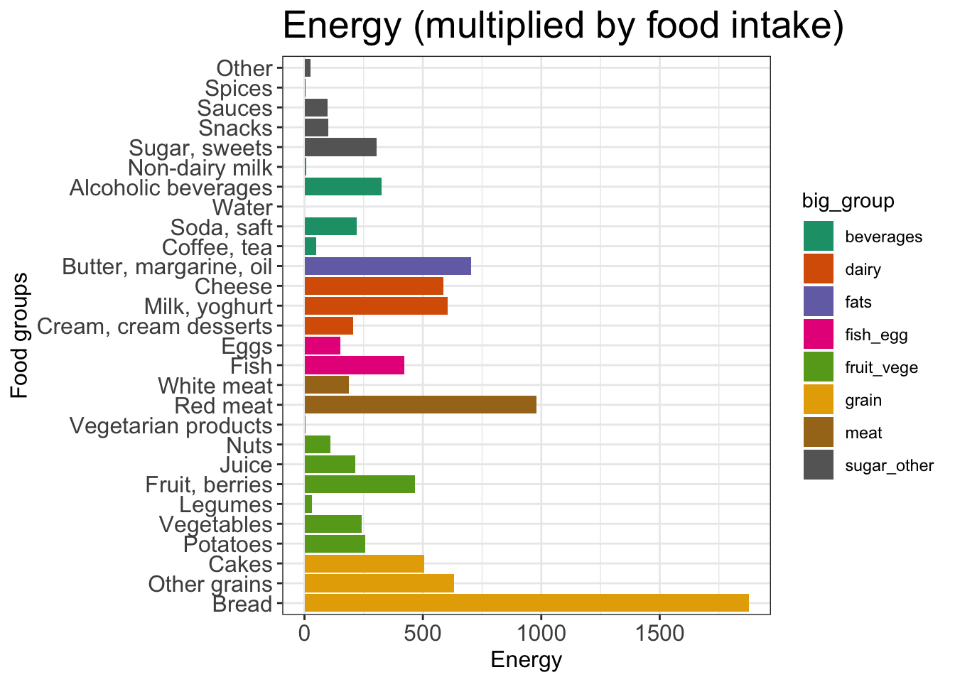
Energy contribution from 28 food groups
In total these 28 food groups contribute to 9314kJ. Here is a breakdown of each food groups, colored by different types of food (crude).
library (ggplot2)library (ggrepel)library (RColorBrewer)<- ggplot (data = pdt_long[category == 'energy' ], aes (x = food_name_order, y = value, fill = big_group))<- p1 + geom_bar (stat = 'identity' )<- p1 + coord_flip ()<- p1 + theme_bw ()<- p1 + scale_fill_brewer (palette = 'Dark2' )<- p1 + labs (title = 'Energy (multiplied by food intake)' , x = 'Food groups' , y = 'Energy' )<- p1 + theme (axis.text = element_text (size = 12 ), axis.title = element_text (size = 12 ), plot.title = element_text (size = 20 ))
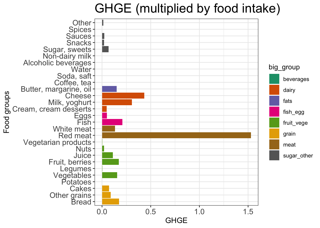
GHGE contribution from 28 food groups
We can also plot a different metric, say GHGE. We can see that red meat is the largest contributor, followed by cheese and milk (dairy products).
Show code
<- ggplot (data = pdt_long[category == 'ghge' ], aes (x = food_name_order, y = value, fill = big_group))<- p2 + geom_bar (stat = 'identity' )<- p2 + coord_flip ()<- p2 + theme_bw ()<- p2 + scale_fill_brewer (palette = 'Dark2' )<- p2 + labs (title = 'GHGE (multiplied by food intake)' , x = 'Food groups' , y = 'GHGE' )<- p2 + theme (axis.text = element_text (size = 12 ), axis.title = element_text (size = 12 ), plot.title = element_text (size = 20 ))
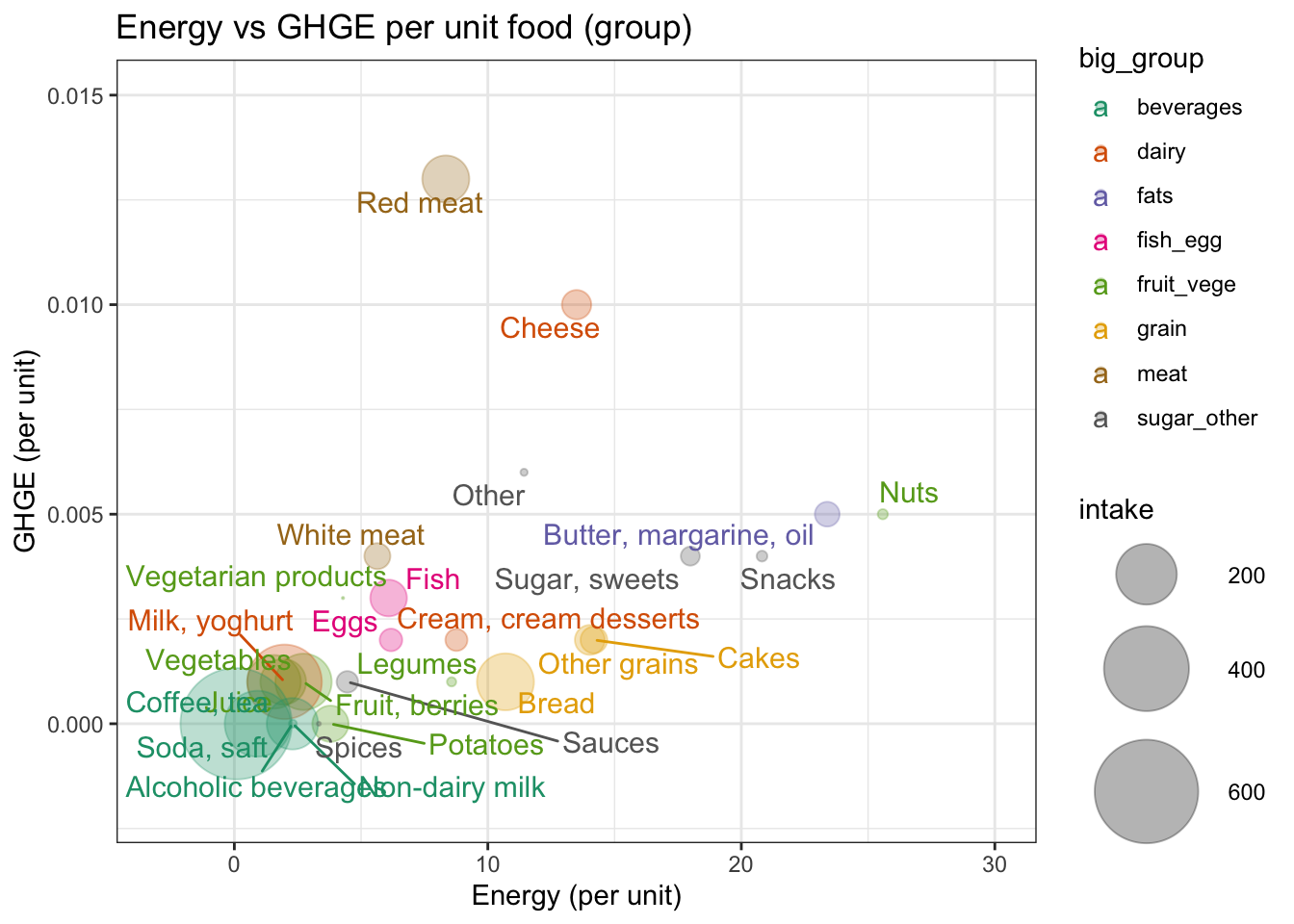
Energy vs GHGE
We can also show the per unit contribution to energy and GHGE. The size of the bubbles are the amount of consumption: the bigger the more consumed.
Show code
<- data.table:: setDT (foods)# remove water, outlier <- pdfd[food != 'Water' ]# attach label %in% grain, big_group : = 'grain' ]%in% fruit_vege, big_group : = 'fruit_vege' ]%in% meat, big_group : = 'meat' ]%in% fish_egg, big_group : = 'fish_egg' ]%in% dairy, big_group : = 'dairy' ]%in% fats, big_group : = 'fats' ]%in% beverages, big_group : = 'beverages' ]%in% sugar_other, big_group : = 'sugar_other' ]<- ggplot (data = pdfd, aes (x = energy, y = ghge, size = intake, label = food, color = big_group))<- p3 + geom_point (alpha = 0.3 ) + xlim (- 3 , 30 ) + ylim (- 0.002 , 0.015 )<- p3 + scale_size (range = c (0.1 , 20 ))<- p3 + geom_text_repel (size = 4 , max.overlaps = 15 )# p3 <- p3 + geom_text(size = 3, check_overlap = T) <- p3 + theme_bw ()<- p3 + scale_color_brewer (palette = 'Dark2' )<- p3 + labs (title = 'Energy vs GHGE per unit food (group)' , x = 'Energy (per unit)' , y = 'GHGE (per unit)' )
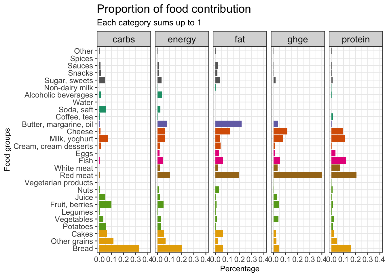
Proportion for 5 metrics
Finally we present the percentage contribution of 28 food groups towards 5 categories.
Show code
<- data.frame (fprop) # total $ food_name <- row.names (pdfp)# attach big group :: setDT (pdfp)%in% grain, big_group : = 'grain' ]%in% fruit_vege, big_group : = 'fruit_vege' ]%in% meat, big_group : = 'meat' ]%in% fish_egg, big_group : = 'fish_egg' ]%in% dairy, big_group : = 'dairy' ]%in% fats, big_group : = 'fats' ]%in% beverages, big_group : = 'beverages' ]%in% sugar_other, big_group : = 'sugar_other' ]<- tidyr:: pivot_longer (pdfp, cols = - c (food_name, big_group), names_to = 'category' )<- data.table:: setDT (pdfp_long)# also add orders here $ food_name_order <- factor (pdfp_long$ food_name, levels = names_ordered, labels = names_ordered)# plot <- ggplot (data = pdfp_long[category %in% c ('energy' , 'protein' , 'fat' , 'carbs' ,'ghge' )], aes (x = food_name_order, y = value, fill = big_group))<- p4 + geom_bar (stat = 'identity' )<- p4 + coord_flip ()<- p4 + facet_wrap (~ category, ncol = 5 )<- p4 + scale_fill_brewer (palette = 'Dark2' )<- p4 + labs (title = 'Proportion of food contribution' ,subtitle = 'Each category sums up to 1' ,x = 'Food groups' , y = 'Percentage' )<- p4 + theme_bw ()<- p4 + theme (axis.text = element_text (size = 10 ), axis.title = element_text (size = 10 ), plot.title = element_text (size = 15 ), strip.text = element_text (size = 12 ), legend.position = 'none' )