# read a csv file, name it 'birth'
# this is the method to read in the data with R command
# you can also use the Rstudio interface to import a dataset
birth <- read.csv('data/birth.csv', sep = ',')Exploratory data analysis (Part I)
Exploring a dataset, descriptive statistics
Datasets
- Explore a dataset:
birth(csv link) - Exercise 1: no data, we type in data directly
- Exercise 2:
PEFH98-english(rda link, csv link)
Explore a dataset
In this section, we will introduce some frequently used commands when you first load a dataset.
We use birth data as an example.
You can type birth in the console to print the data; but you will see that it gets hard to read. This is usually the case: you have lots of data that is hard to fit in your screen.
Therefore, it is useful to
- print out a few rows (head of the data);
- have a list of column names
- know the dimension of the dataset (number of observations and features/measurements)
- produce some summary statistics
We extract the head (first several rows, by default 6) rows of your data. Similarly, you can get the last several rows using tail()
head(birth) id low age lwt eth smk ptl ht ui fvt ttv bwt
1 4 bwt <= 2500 28 120 other smoker 1 no yes 0 0 709
2 10 bwt <= 2500 29 130 white nonsmoker 0 no yes 2 0 1021
3 11 bwt <= 2500 34 187 black smoker 0 yes no 0 0 1135
4 13 bwt <= 2500 25 105 other nonsmoker 1 yes no 0 0 1330
5 15 bwt <= 2500 25 85 other nonsmoker 0 no yes 0 4 1474
6 16 bwt <= 2500 27 150 other nonsmoker 0 no no 0 5 1588# this is giving the first 6 rows of your data
# birth[1:6, ]
# head(birth, 10) gives first 10 rows
# tail(birth)In RStudio, you can also use View() command to look at your dataset in a tabular form.
To know what measurements (or feature, variable, parameter) are in the data, you can extract the column names.
colnames(birth) [1] "id" "low" "age" "lwt" "eth" "smk" "ptl" "ht" "ui" "fvt" "ttv" "bwt"ncol(birth)[1] 12To know how many subjects are in a dataset, there are a few options. You can find the dimension of the dataset; or find how many rows are in the data.
Alternatively, if you have one variable (say age), you can also use length(age).
# by index
birth[1, ]
id low age lwt eth smk ptl ht ui fvt ttv bwt
1 4 bwt <= 2500 28 120 other smoker 1 no yes 0 0 709birth[, 1] [1] 4 10 11 13 15 16 17 18 19 20 22 23 24 25 26 27 28 29
[19] 30 31 32 33 34 35 36 37 40 42 43 44 45 46 47 49 50 51
[37] 52 54 56 57 59 60 61 62 63 65 67 68 69 71 75 76 77 78
[55] 79 81 82 83 84 85 86 87 88 89 91 92 93 94 95 96 97 98
[73] 99 100 101 102 103 104 105 106 107 108 109 111 112 113 114 115 116 117
[91] 118 119 120 121 123 124 125 126 127 128 129 130 131 132 133 134 135 136
[109] 137 138 139 140 141 142 143 144 145 146 147 148 149 150 151 154 155 156
[127] 159 160 161 162 163 164 166 167 168 169 170 172 173 174 175 176 177 179
[145] 180 181 182 183 184 185 186 187 188 189 190 191 192 193 195 196 197 199
[163] 200 201 202 203 204 205 206 207 208 209 210 211 212 213 214 215 216 217
[181] 218 219 220 221 222 223 224 225 226# by column name
birth[, 'age'] [1] 28 29 34 25 25 27 23 24 24 21 32 19 25 16 25 20 21 24 21 20 25 19 19 26 24
[26] 17 20 22 27 20 17 25 20 18 18 20 21 26 31 15 23 20 24 15 23 30 22 17 23 17
[51] 26 20 26 14 28 14 23 17 21 19 33 20 21 18 21 22 17 29 26 19 19 22 30 18 18
[76] 15 25 20 28 32 31 36 28 25 28 17 29 26 17 17 24 35 25 25 29 19 27 31 33 21
[101] 19 23 21 18 18 32 19 24 22 22 23 22 30 19 16 21 30 20 17 17 23 24 28 26 20
[126] 24 28 20 22 22 31 23 16 16 18 25 32 20 23 22 32 30 20 23 17 19 23 36 22 24
[151] 21 19 25 16 29 29 19 19 30 24 19 24 23 20 25 30 22 18 16 32 18 29 33 20 28
[176] 14 28 25 16 20 26 21 22 25 31 35 19 24 45# by $ operator
birth$age [1] 28 29 34 25 25 27 23 24 24 21 32 19 25 16 25 20 21 24 21 20 25 19 19 26 24
[26] 17 20 22 27 20 17 25 20 18 18 20 21 26 31 15 23 20 24 15 23 30 22 17 23 17
[51] 26 20 26 14 28 14 23 17 21 19 33 20 21 18 21 22 17 29 26 19 19 22 30 18 18
[76] 15 25 20 28 32 31 36 28 25 28 17 29 26 17 17 24 35 25 25 29 19 27 31 33 21
[101] 19 23 21 18 18 32 19 24 22 22 23 22 30 19 16 21 30 20 17 17 23 24 28 26 20
[126] 24 28 20 22 22 31 23 16 16 18 25 32 20 23 22 32 30 20 23 17 19 23 36 22 24
[151] 21 19 25 16 29 29 19 19 30 24 19 24 23 20 25 30 22 18 16 32 18 29 33 20 28
[176] 14 28 25 16 20 26 21 22 25 31 35 19 24 45# what column names are there?
colnames(birth) [1] "id" "low" "age" "lwt" "eth" "smk" "ptl" "ht" "ui" "fvt" "ttv" "bwt"# how many columns and rows?
ncol(birth)[1] 12nrow(birth)[1] 189dim(birth)[1] 189 12Sometimes it is also useful to know what types of data it is for each variable. You can either use str() (structure) on the dataset; or use class() on the variable you are interested in.
str(birth)'data.frame': 189 obs. of 12 variables:
$ id : int 4 10 11 13 15 16 17 18 19 20 ...
$ low: chr "bwt <= 2500" "bwt <= 2500" "bwt <= 2500" "bwt <= 2500" ...
$ age: int 28 29 34 25 25 27 23 24 24 21 ...
$ lwt: int 120 130 187 105 85 150 97 128 132 165 ...
$ eth: chr "other" "white" "black" "other" ...
$ smk: chr "smoker" "nonsmoker" "smoker" "nonsmoker" ...
$ ptl: int 1 0 0 1 0 0 0 1 0 0 ...
$ ht : chr "no" "no" "yes" "yes" ...
$ ui : chr "yes" "yes" "no" "no" ...
$ fvt: int 0 2 0 0 0 0 1 1 0 1 ...
$ ttv: int 0 0 0 0 4 5 5 2 5 4 ...
$ bwt: int 709 1021 1135 1330 1474 1588 1588 1701 1729 1790 ...class(birth$age)[1] "integer"class(birth$low)[1] "character"Descriptive statistics
Continuous variable
A continuous variable can take values in a continuous range. Height and weight are examples of this type. Usually the data type in R is numeric; if not, you might need to convert it first.
Common summary statistics for continuous variables are
- extremes (minimum, maximum)
- average and central tendency (mean, median)
- quantiles (top 1 percent, bottom 5 percent, IQR - interquartile range)
Let us focus on one continuous variable, bill_length_mm.
# create a variable called age
age <- birth$age


# use the command summary on a continuous variable
summary(age)
Min. 1st Qu. Median Mean 3rd Qu. Max.
14.00 19.00 23.00 23.24 26.00 45.00 # compute the min, max
min(age)[1] 14max(age)[1] 45mean(age)[1] 23.2381median(age)[1] 23quantile(age, 0.05)5%
16 quantile(age, 0.95)95%
32 Categorical variable
Categorical variables take discrete values, such as sex (male and female), smoking habit (frequent smoker or not), age groups.
For categorical variables, the metrics above (mean and median, max and min, quantiles) do not make much sense. We use counts and percentages instead.
We use the variable species and island from the penguin data.
# categorical variable
smoker <- birth$smk
low_birthweight <- birth$low

# categories with counts
table(smoker)
smoker
nonsmoker smoker
115 74 table(low_birthweight)low_birthweight
bwt <= 2500 bwt > 2500
59 130 # two categories
table(smoker, low_birthweight) low_birthweight
smoker bwt <= 2500 bwt > 2500
nonsmoker 29 86
smoker 30 44# to create percentage, divide by number of subjects
table(smoker)/length(smoker)smoker
nonsmoker smoker
0.6084656 0.3915344 Visualization
Histogram
hist(age)
Box plot
A boxplot gives the position of
- median (50th percentile; second quartile)
- 25th and 75th percentile (first and third quartile)
- maximum and minimum
- outliers
boxplot(age)
# multiple boxplot together
boxplot(bwt ~ smk, data = birth)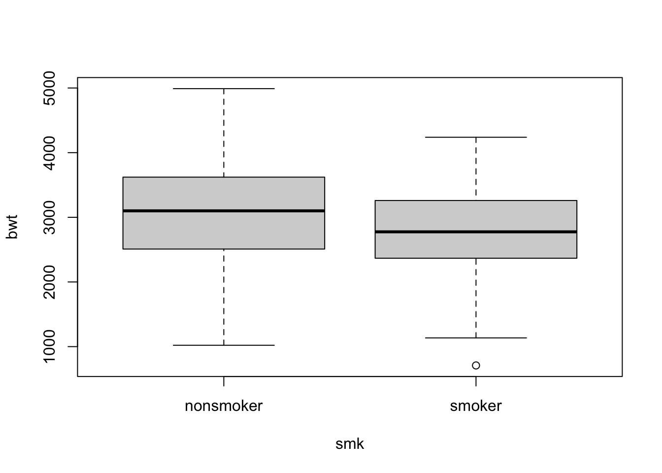
Scatterplot of two continuous variables
plot(birth$age, birth$bwt)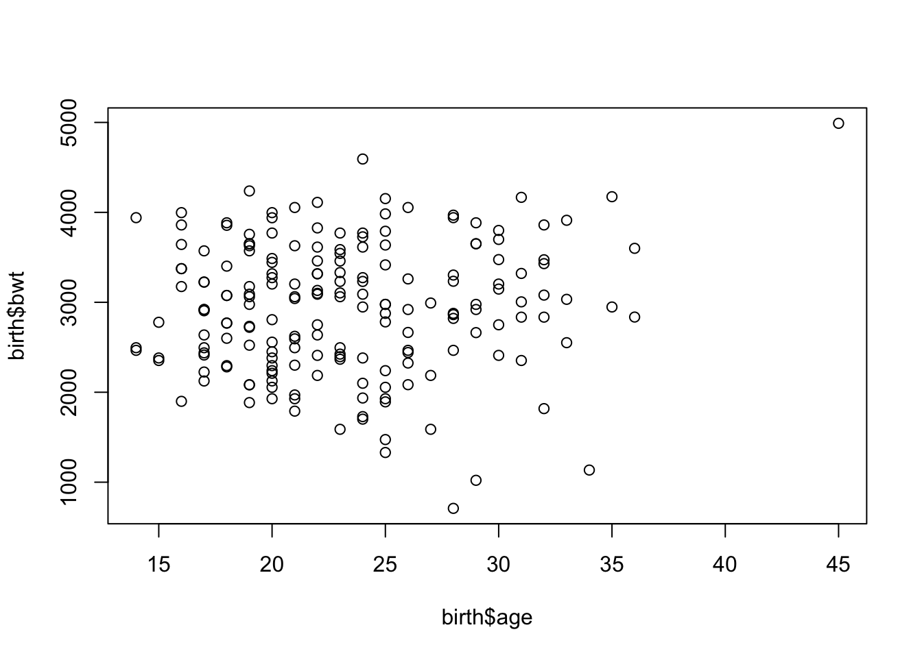
Exercise 1 (weight)
1a
Generate a variable named weight, with the following measurements:
50 75 70 74 95 83 65 94 66 65 65 75 84 55 73 68 72 67 53 651b
Make a simple descriptive analysis of the variable, what are the mean, standard deviation, maximum, minimum and quantiles?
How to interpret the data?
1c
Make a histogram.
1d
Make a boxplot. What do the two dots on the top represent?
Exercise 2 (lung function)
Lung function has been measured on 106 medical students. Peak expiratory flow rate (PEF, measured in liters per minute) was measured three times in a sittinng position, and three times in a standing position.
The variables are
- Age (years)
- Gender (1 is female, 2 is male)
- Height (cm)
- Weight (kg)
- PEF measured three times in a sitting position (pefsit1, pefsit2, pefsit3)
- PEF measured three times in a standing position (pefsta1, pefsta2, pefsta3)
- Mean of the three measurements made in a sitting position (pefsitm)
- Mean of the three measurements made in a standing position (pefstam)
- Mean of all six PEF values (pefmean)
2a)
Download and open PEFH98-english.dta into R.
If you have problem with .dta data format, you can also use PEFH98-english.csv.
Pay attention to how gender is coded. We might have to modify it.
2b)
How many observations are there (number of subjects)? How do you get a list of variable names from your dataset?
Make a histogram for each of the following variables. Compute means, and interpret the results.
height
weight
age
pefsitm
pefstam
2c)
Make histograms for the variables height and pefmean for men and women separately. Also try to make boxplots.
What conclusion can you draw?
2d)
Make three scatterplots to compare
pefmeanwithheightpefmeanwithweightpefmeanwithage
What association do you see?
Solution
Exercise 1 (weight)
1a
Generate a variable named weight, with the following measurements:
50 75 70 74 95 83 65 94 66 65 65 75 84 55 73 68 72 67 53 65weight <- c(50, 75, 70, 74, 95,
83, 65, 94, 66, 65,
65, 75, 84, 55, 73,
68, 72, 67, 53, 65)1b
Make a simple descriptive analysis of the variable, what are the mean, median, maximum, minimum and quantiles?
How to interpret the data?
mean(weight)[1] 70.7median(weight)[1] 69max(weight)[1] 95min(weight)[1] 50# alternatively,
summary(weight) Min. 1st Qu. Median Mean 3rd Qu. Max.
50.0 65.0 69.0 70.7 75.0 95.0 1c
Make a histogram.
hist(weight)
1d
Make a boxplot. What do the two dots on the top represent?
boxplot(weight)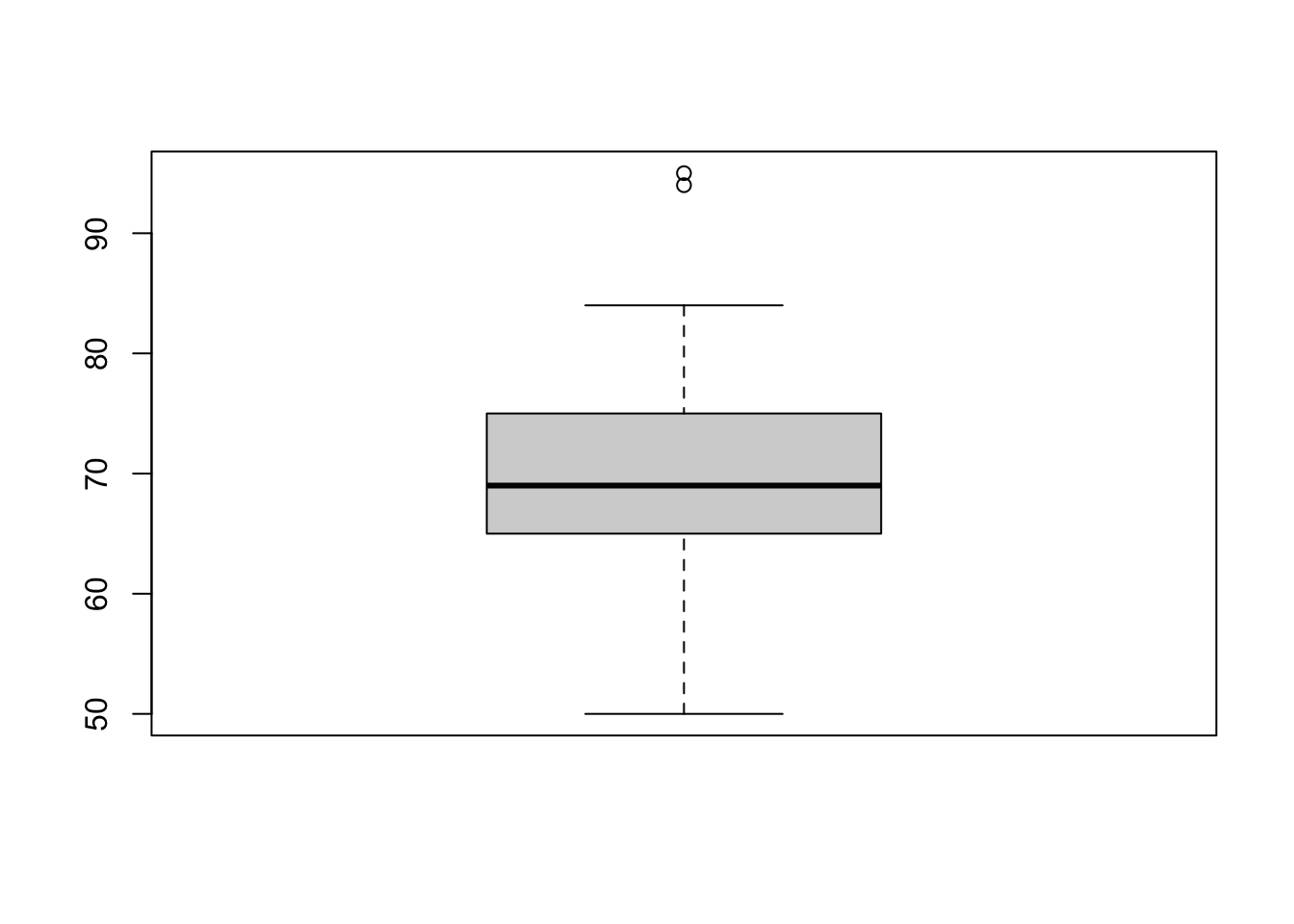
They are the largest two points in the dataset. These are outliers in this data.
(Optional) Outliers in box plot
There are different ways to define outliers. The default box plot in R determines points beyond \(Q_1 - 1.5\times IQR\) and \(Q_3 + 1.5\times IQR\) are outliers. You can check the values of quartiles using summary(), and read up the documentation ?boxplot().
Exercise 2 (lung function)
Lung function has been measured on 106 medical students. Peak expiratory flow rate (PEF, measured in liters per minute) was measured three times in a sittinng position, and three times in a standing position.
The variables are
- Age (years)
- Gender (1 is female, 2 is male)
- Height (cm)
- Weight (kg)
- PEF measured three times in a sitting position (pefsit1, pefsit2, pefsit3)
- PEF measured three times in a standing position (pefsta1, pefsta2, pefsta3)
- Mean of the three measurements made in a sitting position (pefsitm)
- Mean of the three measurements made in a standing position (pefstam)
- Mean of all six PEF values (pefmean)
2a)
Download and open PEFH98-english.dta into R.
If you have problem with .dta data format, you can also use PEFH98-english.csv.
Pay attention to how gender is coded. We might have to modify it.
# locate your datafile, set the path to your data
# if you use rda data file:
# load('./lab/data/PEFH98-english.rda')

# if you use csv:
lung_data <- read.csv('data/PEFH98-english.csv', sep = ',')
head(lung_data)
age gender height weight pefsit1 pefsit2 pefsit3 pefsta1 pefsta2 pefsta3
1 20 female 165 50 400 400 410 410 410 400
2 20 male 185 75 480 460 510 520 500 480
3 21 male 178 70 490 540 560 470 500 470
4 21 male 179 74 520 530 540 480 510 500
5 20 male 196 95 740 750 750 700 710 700
6 20 male 189 83 600 575 600 600 600 640
pefsitm pefstam pefmean
1 403.3333 406.6667 405.0000
2 483.3333 500.0000 491.6667
3 530.0000 480.0000 505.0000
4 530.0000 496.6667 513.3333
5 746.6667 703.3333 725.0000
6 591.6667 613.3333 602.50002b)
How many observations are there (number of subjects)? How do you get a list of variable names from your dataset?
nrow(lung_data)[1] 106colnames(lung_data) [1] "age" "gender" "height" "weight" "pefsit1" "pefsit2" "pefsit3"
[8] "pefsta1" "pefsta2" "pefsta3" "pefsitm" "pefstam" "pefmean"Make a histogram for each of the following variables. Compute means, and interpret the results.
height
weight
age
pefsitm
pefstamhist(lung_data$height)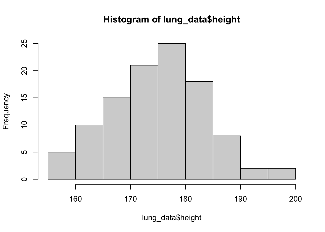
We repeat it for the other 4 variables. We can put them more compactly,
par(mfrow = c(2, 2))
# we use this line to display (2 rows 2 columns)
# by default it is 1 row 1 column
# run this line to set it back to default:
# par(mfrow = c(1, 1))
hist(lung_data$weight)
hist(lung_data$age)
hist(lung_data$pefsitm)
hist(lung_data$pefstam)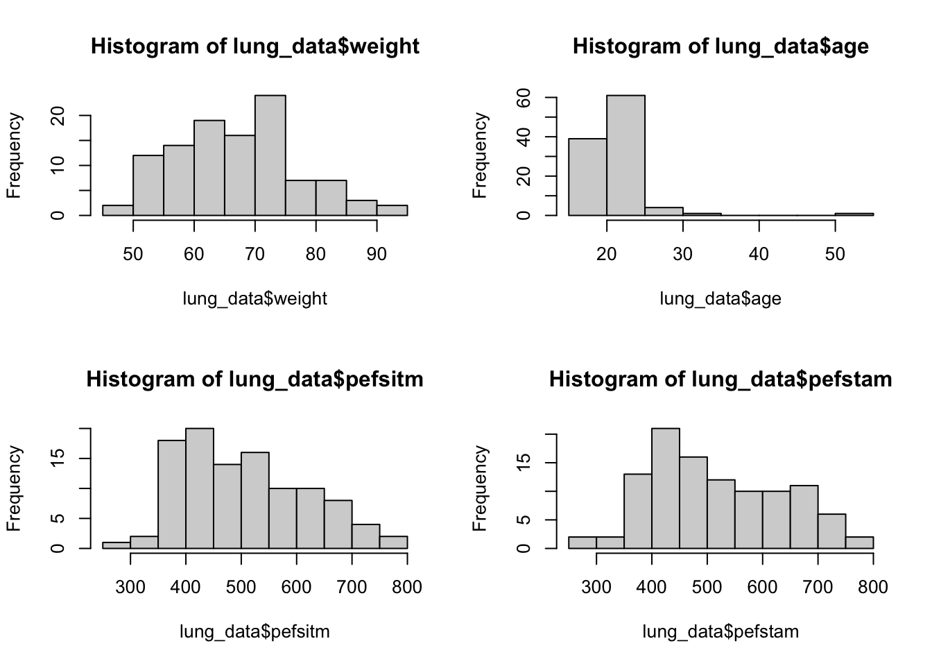
2c)
Make histograms for the variables height and pefmean for men and women separately. Also try to make boxplots.
What conclusion can you draw?
height_f <- lung_data$height[lung_data$gender == 'female']
height_m <- lung_data$height[lung_data$gender == 'male']

par(mfrow = c(1,2)) # plot in parallel
hist(height_f)
hist(height_m)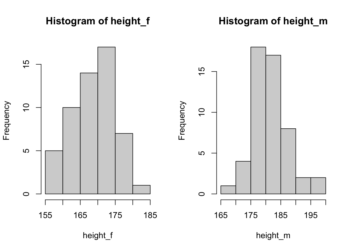
# we can make it more customized
# add axis limit, title and xaxis name
par(mfrow = c(1,2)) # plot in parallel
hist(height_f, main = 'Height: female', xlab = 'Height (cm)',
     xlim = c(150, 200))
hist(height_m, main = 'Height: male', xlab = 'Height (cm)',
     xlim = c(150, 200))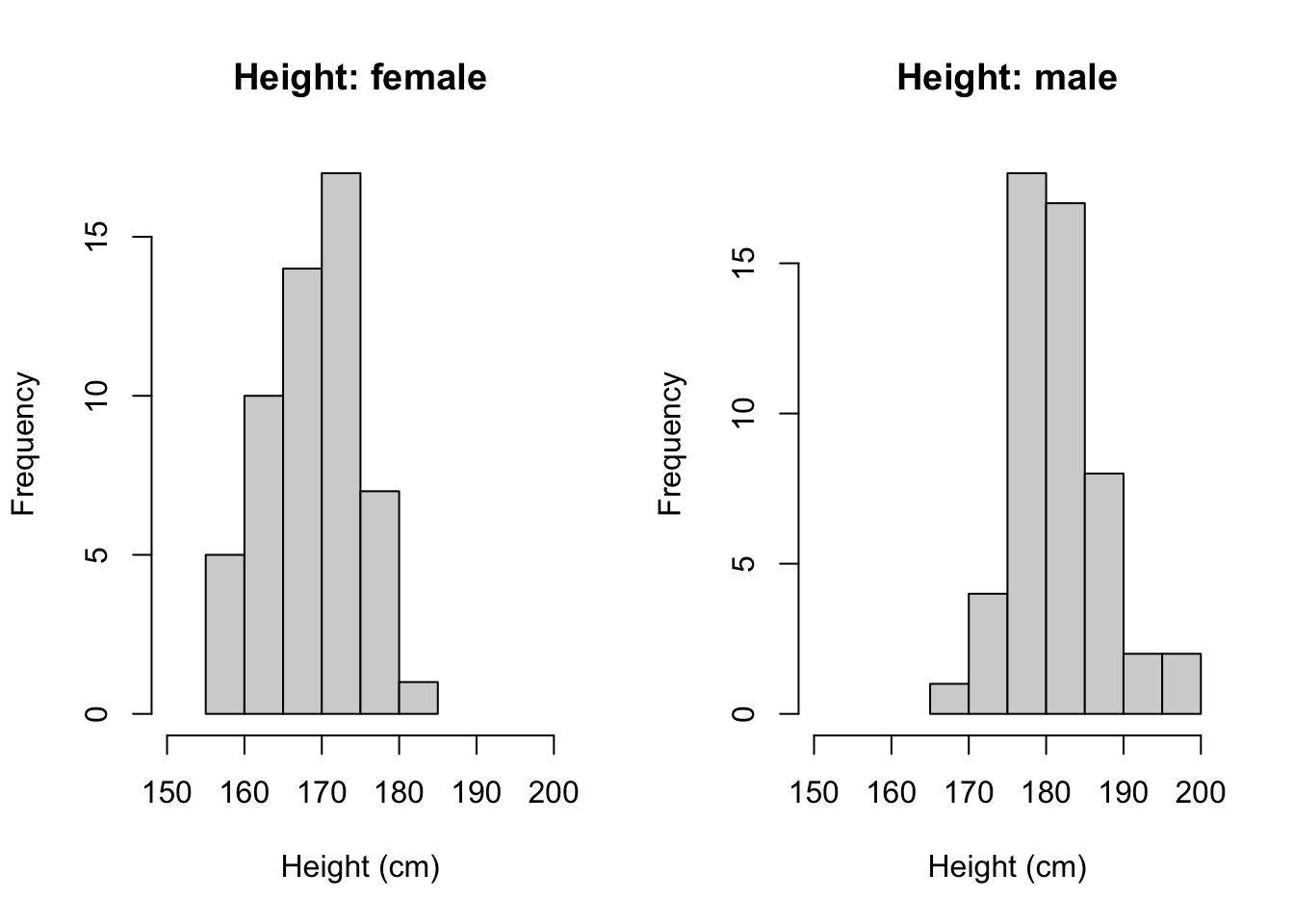
Similarly, histogram for pefmean can be done in the same way.
pefmean_f <- lung_data$pefmean[lung_data$gender == 'female']
pefmean_m <- lung_data$pefmean[lung_data$gender == 'male']

par(mfrow = c(1,2)) # plot in parallel
hist(pefmean_f)
hist(pefmean_m)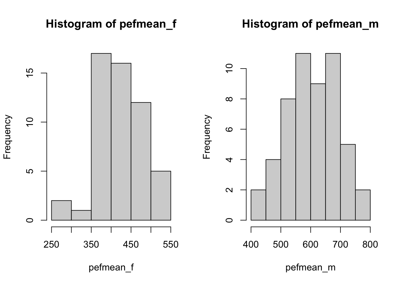
Now we can make some boxplots
par(mfrow = c(1, 2))
boxplot(height ~ gender, data = lung_data, main = 'Height vs Gender')

# it is also possible to remove the frame
boxplot(pefmean ~ gender, data = lung_data, frame = F, main = 'PEFmean vs gender')
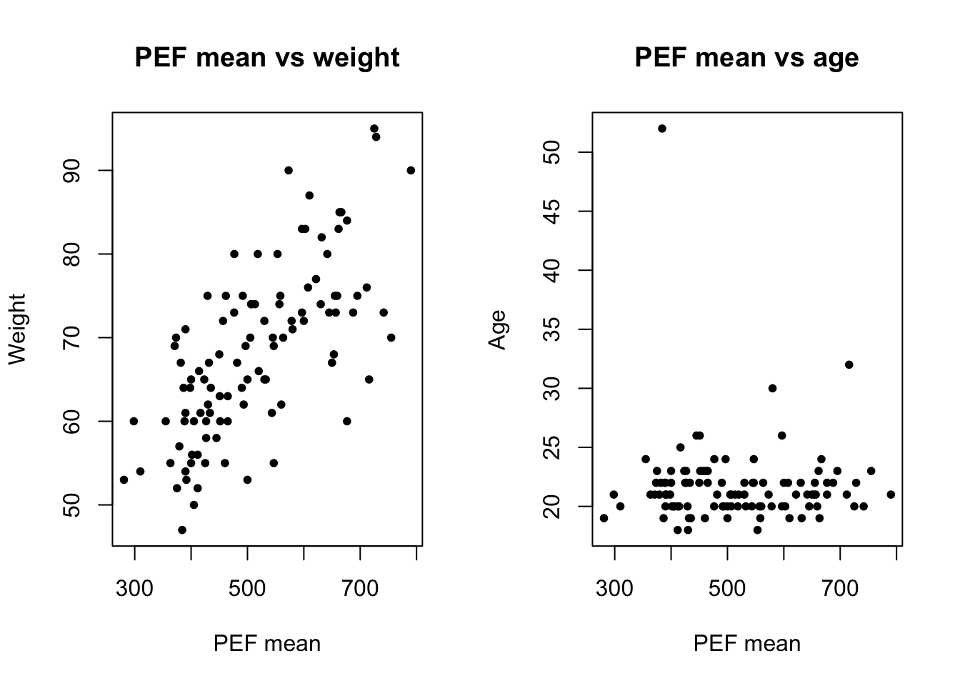
2d)
Make three scatterplots to compare
pefmeanwithheightpefmeanwithweightpefmeanwithage
What association do you see?
# pefmean height
plot(lung_data$pefmean, lung_data$height)
# it is possible to customize
plot(lung_data$pefmean, lung_data$height,
     main = 'PEF mean vs height',
     xlab = 'PEF mean', ylab = 'Height',
     pch = 20)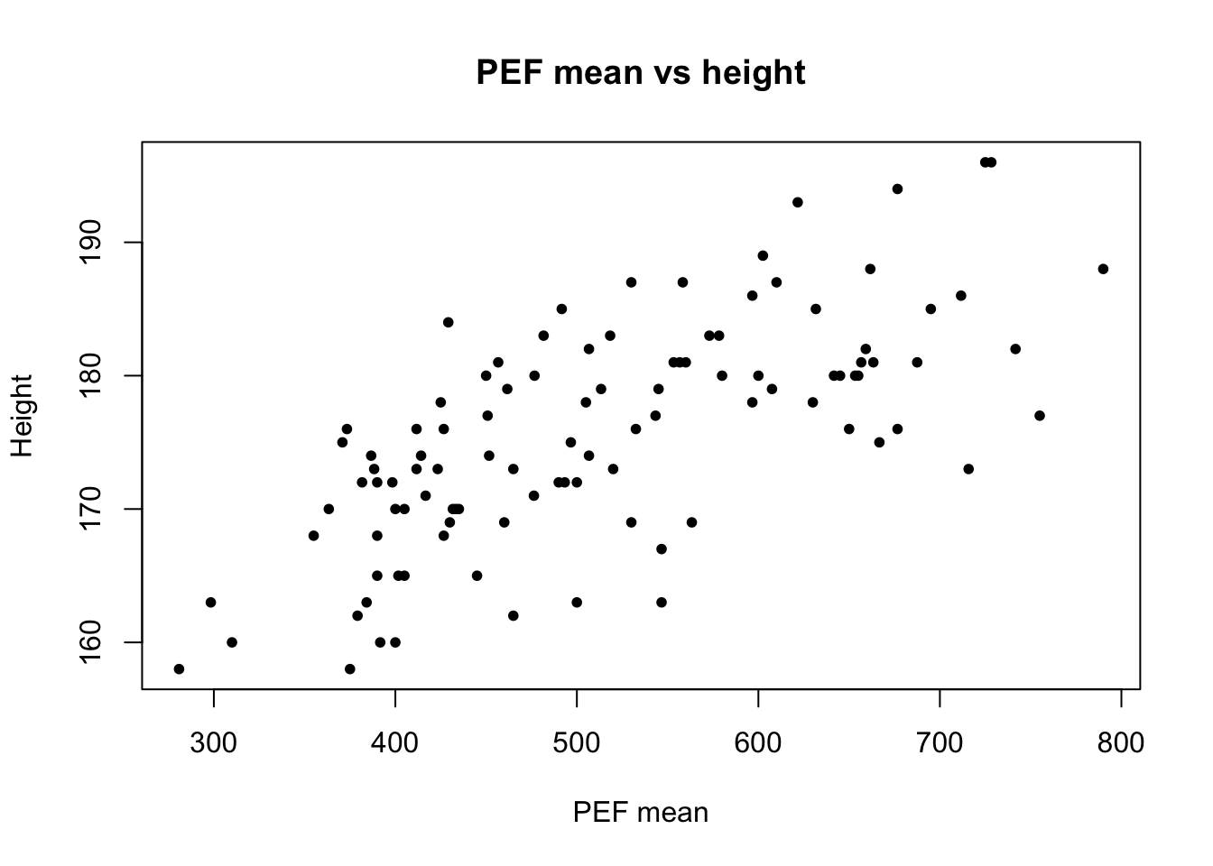
# pch: plotting symbolspch = 20 is setting the symbol to small solid dots. You can try different values, from 0 to 25. Read more
par(mfrow = c(1, 2))
# pefmean weight
plot(lung_data$pefmean, lung_data$weight,
     main = 'PEF mean vs weight',
     xlab = 'PEF mean', ylab = 'Weight',
     pch = 20)

# pefmean age
plot(lung_data$pefmean, lung_data$age,
     main = 'PEF mean vs age',
     xlab = 'PEF mean', ylab = 'Age',
     pch = 20)