Survival analysis

Kaplan-Meier curve, log rank tests

Datasets

Exercise 1: melanoma(rda link, csv link)
Exercise 2: liggetid (rda link, csv link)

Exercise 1: Melanoma

The data concern 205 patients with malignant melanoma who were operated at the university hospital in Odense, Denmark, in the period 1962-77. The patients were followed up to death or censored at the end of the study. We shall study the effect on survival of the patient’s gender and tumor thickness.

The variables included in the dataset are:

status (1=death from disease, 2=censored, 4=death from other causes)
lifetime (years) from operation
ulceration of tumor (1=yes, 2=no)
tumor thickness in 1/100 mm
gender (f=1, m=2)
age at operation in years
grouped tumor thickness (1: 0-1 mm, 2: 2-5 mm, 3: 5+ mm)
logarithm of tumor thickness

1a)

The “event of interest” is defined as “death from disease”. Pre-process the variables that R will use for basic survival analysis as shown in class.

1b)

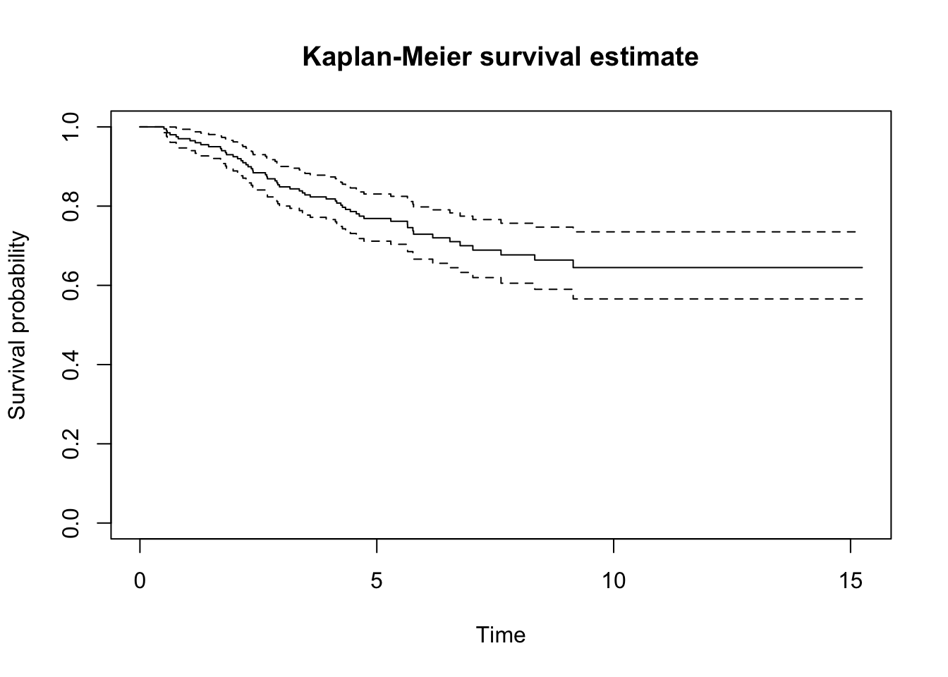
Make a Kaplan-Meier plot of the survival curve. What are the estimated probabilities of surviving 1 year, 2 years, 5 years?

1c)

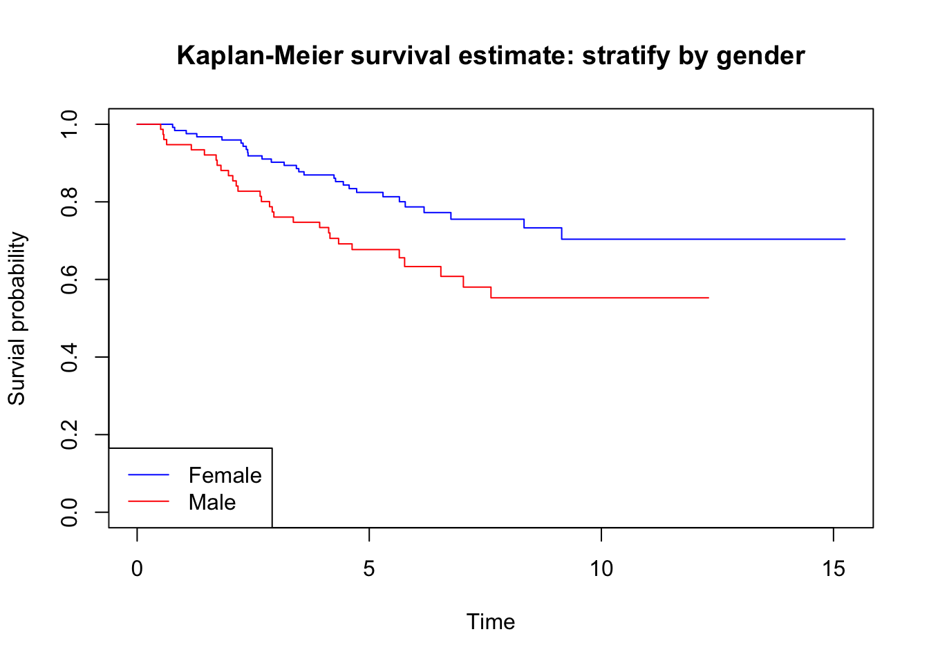
Compare survival according to gender. Test the difference with a logrank test.

1d)

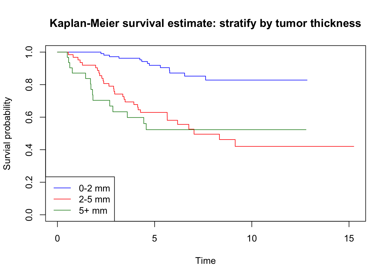
Study survival according to grouped tumor thickness by comparing survival curves in each group and test with a logrank test.

Exercise 2: length of hospital stay

The data was collected at the Geriatric Department at Ullevål Sykehus. Below is a description of the data set liggetid. The file includes the following variables:

Year of birth (faar)
Month of birth (fmaan)
Day of birth (fdag)
Year of hospital admission (innaar)
Month of admission (innmaan)
Day of admission (inndag)
Year of discharge from hospital (utaar)
Month of discharge (utmaan)
Day of discharge (utdag)
Gender, where 1 = male and 0 = female (kjoenn)
Admission from, where 1 = home, 2 = Div. of Medicine, 3 = Div. of Surgery, 4 = Other division, 5 = Other hospital, 6 = Nursing home (kom_fra)
Stroke, where 1 = yes, 0 = no (slag)
Age (alder)
Hospital stay, in days (liggetid)
Logarithm of hospital stay (lnliggti)
Comes from Div. of Medicine (kom_fra2)
Comes from Div. of Surgery (kom_fra3)
Comes from Other division (kom_fra4)
Comes from Other hospital (kom_fra5)
Comes from Nursing home (kom_fra6)
Censoring variable (censor)

The variable liggetid time is calculated from the innaar, innmaan, inndag, utaar, utmaan and utdag variables.

2a)

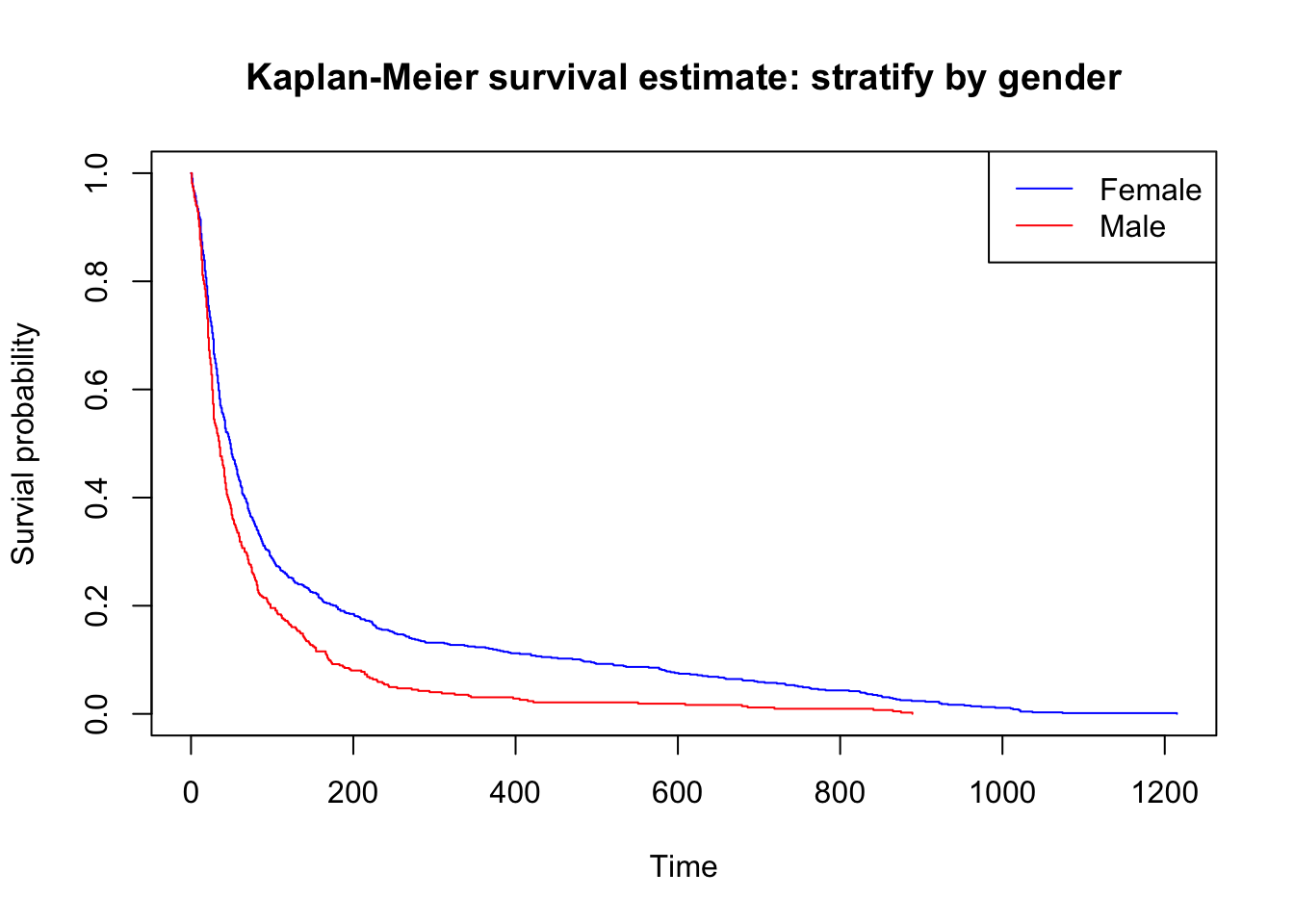
Analyze the relationship between the variables liggetid and kjoenn with a Kaplan-Meier plot. Test the difference with a log-rank test.

2b)

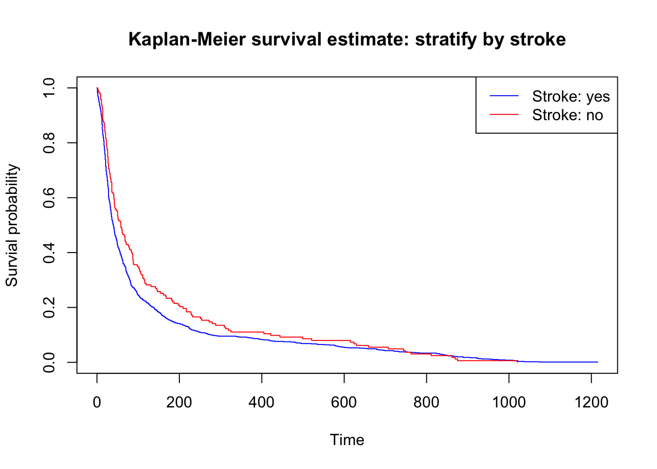
Analyze the relationship between the variables liggetid and slag with a Kaplan-Meier plot. Test the difference with a log-rank test.

Solution

Exercise 1: Melanoma

The variables included in the dataset are:

status (1=death from disease, 2=censored, 4=death from other causes)
lifetime (years) from operation
ulceration of tumor (1=yes, 2=no)
tumor thickness in 1/100 mm
gender (f=1, m=2)
age at operation in years
grouped tumor thickness (1: 0-1 mm, 2: 2-5 mm, 3: 5+ mm)
logarithm of tumor thickness

First we load the dataset, and check what columns are there.

# if you do not have survival package, install it by 
# install.packages('survival')
library(survival)

melanoma <- read.csv('data/melanoma.csv')

head(melanoma)

  status   lifetime ulceration tumor_thickness gender age
1      4 0.02739726        Yes            6.76      m  76
2      4 0.08219178         No            0.65      m  56
3      2 0.09589041         No            1.34      m  41
4      4 0.27123288         No            2.90      f  71
5      1 0.50684932        Yes           12.08      m  52
6      1 0.55890411        Yes            4.84      m  28
  grouped_tumor_thickness logarithm_of_tumor_thickness
1                   5+ mm                    1.9110229
2                  0-2 mm                   -0.4307829
3                  0-2 mm                    0.2926696
4                  2-5 mm                    1.0647107
5                   5+ mm                    2.4915512
6                  2-5 mm                    1.5769147

colnames(melanoma)

[1] "status"                       "lifetime"                    
[3] "ulceration"                   "tumor_thickness"             
[5] "gender"                       "age"                         
[7] "grouped_tumor_thickness"      "logarithm_of_tumor_thickness"

1a)

The “event of interest” is defined as “death from disease”. Pre-process the variables that R will use for basic survival analysis as shown in class.

We only need “death from melanoma” or else, hence we need to recode the status variable which originally had three categories.

# if status == 1, code 1; otherwise, code 0
# this indicates whether deaths from melanoma
death <- ifelse(melanoma$status == 1, 1, 0)

# check if the labels are correct
table(death)

death
  0   1 
148  57

table(melanoma$status)


  1   2   4 
 57 134  14

You can see that the category melanoma$status == 1 should match death == 1, and melanoma$status of 2 and 4 are merged together and coded as death == 0.

1b)

Make a Kaplan-Meier plot of the survival curve. What are the estimated probabilities of surviving 1 year, 2 years, 5 years?

# take lifetime variable
lifetime <- melanoma$lifetime

km_fit <- survfit(Surv(lifetime, death) ~ 1)
plot(km_fit)

# add title and text
title(main = 'Kaplan-Meier survival estimate', 
      xlab = 'Time', 
      ylab = 'Survival probability')

Now we check only time 1, 2, 5.

# time 1, 2, 5
tme <- c(1, 2, 5)
summary(km_fit, times = tme)

Call: survfit(formula = Surv(lifetime, death) ~ 1)

 time n.risk n.event survival std.err lower 95% CI upper 95% CI
    1    193       6    0.970  0.0120        0.947        0.994
    2    183       9    0.925  0.0187        0.889        0.962
    5    122      30    0.769  0.0303        0.712        0.831

1c)

Compare survival according to gender. Test the difference with a logrank test.

# gender == 1: female; gender == 2: male
gender <- melanoma$gender

km_fit_gender <- survfit(Surv(lifetime, death) ~ gender)
plot(km_fit_gender, col = c('blue', 'red'))
title(main = 'Kaplan-Meier survival estimate: stratify by gender', 
      xlab = 'Time', 
      ylab = 'Survial probability')

# add legend
legend( 'bottomleft', 
       legend = c('Female', 'Male'), 
       lty = c('solid', 'solid'), 
       col = c('blue','red'))

Now we test the difference with log-rank test

# test difference with logrank test 
survdiff(Surv(lifetime, death) ~ gender)

Call:
survdiff(formula = Surv(lifetime, death) ~ gender)

           N Observed Expected (O-E)^2/E (O-E)^2/V
gender=f 126       28     37.1      2.25      6.47
gender=m  79       29     19.9      4.21      6.47

 Chisq= 6.5  on 1 degrees of freedom, p= 0.01

1d)

Study survival according to grouped tumor thickness by comparing survival curves in each group and test with a logrank test.

First we do some data processing

# take out the variable
grouped_tumor_thickness <- melanoma$grouped_tumor_thickness

# get an idea how many categories
table(grouped_tumor_thickness)

grouped_tumor_thickness
0-2 mm 2-5 mm  5+ mm 
   109     64     32

Now we plot the KM plot, and carry out a log-rank test

km_fit_tumor <- survfit(Surv(lifetime, death) ~ grouped_tumor_thickness)
plot(km_fit_tumor, col = c('blue', 'red', 'forestgreen'))

title(main = 'Kaplan-Meier survival estimate: stratify by tumor thickness', 
      xlab = 'Time', 
      ylab = 'Survial probability')

# add legend
legend( 'bottomleft', 
        legend = c('0-2 mm', '2-5 mm', '5+ mm'), 
        lty = c('solid', 'solid', 'solid'), 
        col = c('blue','red', 'forestgreen'))

# test difference with logrank test 
survdiff(Surv(lifetime, death) ~ grouped_tumor_thickness)

Call:
survdiff(formula = Surv(lifetime, death) ~ grouped_tumor_thickness)

                                 N Observed Expected (O-E)^2/E (O-E)^2/V
grouped_tumor_thickness=0-2 mm 109       13    33.75     12.75     31.36
grouped_tumor_thickness=2-5 mm  64       30    16.39     11.30     15.88
grouped_tumor_thickness=5+ mm   32       14     6.86      7.42      8.45

 Chisq= 31.6  on 2 degrees of freedom, p= 1e-07

Exercise 2: Length of hospital stay

The data was collected at the Geriatric Department at Ullevål Sykehus. Below is a description of the data set liggetid. The file includes the following variables:

Year of birth (faar)
Month of birth (fmaan)
Day of birth (fdag)
Year of hospital admission (innaar)
Month of admission (innmaan)
Day of admission (inndag)
Year of discharge from hospital (utaar)
Month of discharge (utmaan)
Day of discharge (utdag)
Gender, where 1 = male and 0 = female (kjoenn)
Admission from, where 1 = home, 2 = Div. of Medicine, 3 = Div. of Surgery, 4 = Other division, 5 = Other hospital, 6 = Nursing home (kom_fra)
Stroke, where 1 = yes, 0 = no (slag)
Age (alder)
Hospital stay, in days (liggetid)
Logarithm of hospital stay (lnliggti)
Comes from Div. of Medicine (kom_fra2)
Comes from Div. of Surgery (kom_fra3)
Comes from Other division (kom_fra4)
Comes from Other hospital (kom_fra5)
Comes from Nursing home (kom_fra6)
Censoring variable (censor)

The variable liggetid time is calculated from the innaar, innmaan, inndag, utaar, utmaan and utdag variables.

liggetid <- read.csv('data/liggetid.csv')
head(liggetid)

  faar fmaan fdag innaar innmaan inndag utaar utmaan utdag kjoenn kom_fra slag
1 1906     3    4   1987       3      5    87      3    18 kvinne       1    0
2 1891     4    3   1987       3      6    87      3    23 kvinne       1    0
3 1908     9    6   1987       3     10    87      3    16 kvinne       1    0
4 1910     1   11   1987       3     11    87      3    25   mann       1    1
5 1907     1    6   1987       3     13    87      3    30 kvinne       1    0
6 1901    12   19   1987       3     13    87      4     2 kvinne       1    0
  alder liggetid lnliggti kom_fra2 kom_fra3 kom_fra4 kom_fra5 kom_fra6 status
1    81       13 2.564949        0        0        0        0        0      1
2    96       17 2.833213        0        0        0        0        0      1
3    79        6 1.791759        0        0        0        0        0      1
4    77       14 2.639057        0        0        0        0        0      1
5    80       17 2.833213        0        0        0        0        0      1
6    86       20 2.995732        0        0        0        0        0      1

colnames(liggetid)

 [1] "faar"     "fmaan"    "fdag"     "innaar"   "innmaan"  "inndag"  
 [7] "utaar"    "utmaan"   "utdag"    "kjoenn"   "kom_fra"  "slag"    
[13] "alder"    "liggetid" "lnliggti" "kom_fra2" "kom_fra3" "kom_fra4"
[19] "kom_fra5" "kom_fra6" "status"

# all status are 1 
status <- liggetid$status

2a)

Analyze the relationship between the variables liggetid and kjoenn with a Kaplan-Meier plot. Test the difference with a log-rank test.

# length of stay (los) vs gender
los <- liggetid$liggetid
head(los)

[1] 13 17  6 14 17 20

# take out gender variable
gender <- liggetid$kjoenn
head(gender)

[1] "kvinne" "kvinne" "kvinne" "mann"   "kvinne" "kvinne"

# fit km 
km_liggetid_gender <- survfit(Surv(los, status) ~ gender)

plot(km_liggetid_gender, col = c('blue', 'red'))

title(main = 'Kaplan-Meier survival estimate: stratify by gender', 
      xlab = 'Time', 
      ylab = 'Survial probability')

# add legend
legend( 'topright', 
        legend = c('Female', 'Male'), 
        lty = c('solid', 'solid'), 
        col = c('blue','red'))

Now we do log-rank test

# log rank test 
survdiff(Surv(los, status) ~ gender)

Call:
survdiff(formula = Surv(los, status) ~ gender)

n=1138, 1 observation deleted due to missingness.

                N Observed Expected (O-E)^2/E (O-E)^2/V
gender=kvinne 714      714      799      9.06      31.9
gender=mann   424      424      339     21.36      31.9

 Chisq= 31.9  on 1 degrees of freedom, p= 2e-08

2b)

Analyze the relationship between the variables liggetid and slag with a Kaplan-Meier plot. Test the difference with a log-rank test.

# length of stay vs stroke
# slag == 1: yes, slag == 2: no
stroke <- liggetid$slag

# fit km 
km_liggetid_stroke <- survfit(Surv(los, status) ~ stroke)

plot(km_liggetid_stroke, col = c('blue', 'red'))

title(main = 'Kaplan-Meier survival estimate: stratify by stroke', 
      xlab = 'Time', 
      ylab = 'Survial probability')

# add legend
legend( 'topright', 
        legend = c('Stroke: yes', 'Stroke: no'), 
        lty = c('solid', 'solid'), 
        col = c('blue','red'))

# log rank test
survdiff(Surv(los, status) ~ stroke)

Call:
survdiff(formula = Surv(los, status) ~ stroke)

n=1054, 85 observations deleted due to missingness.

           N Observed Expected (O-E)^2/E (O-E)^2/V
stroke=0 891      891      864     0.814      4.61
stroke=1 163      163      190     3.714      4.61

 Chisq= 4.6  on 1 degrees of freedom, p= 0.03