The Truncated Exponential Family

Random generation for the truncated exponential family distributions. Please ferer to the "Details" and "Examples" section for more information on how to use this function.

Usage

rtrunc(n, family = "gaussian", faster = FALSE, ...)

rtrunc.beta(n, shape1, shape2, a = 0, b = 1)

rtruncbeta(n, shape1, shape2, a = 0, b = 1)

rtruncbinom(n, size, prob, a = 0, b = size)

rtruncchisq(n, df, a = 0, b = Inf)

rtrunccontbern(n, lambda, a = 0, b = 1)

rtruncexp(n, rate = 1, a = 0, b = Inf)

rtruncgamma(n, shape, rate = 1, scale = 1/rate, a = 0, b = Inf)

rtruncinvgamma(n, shape, rate = 1, scale = 1/rate, a = 0, b = Inf)

rtruncinvgauss(n, m, s, a = 0, b = Inf)

rtrunclnorm(n, meanlog, sdlog, a = 0, b = Inf)

rtruncnbinom(n, size, prob, mu, a = 0, b = Inf)

rtruncnorm(n, mean, sd, a = -Inf, b = Inf)

rtruncpois(n, lambda, a = 0, b = Inf)

rtrunc_direct(n, family = "gaussian", parms, ...)

Arguments

n

sample size

family

distribution family to use

faster

if TRUE, samples directly from the truncated distribution (more info in details)

...

individual arguments to each distribution

shape1

positive shape parameter alpha

shape2

positive shape parameter beta

a

point of left truncation

b

point of right truncation

size

target for number of successful trials, or dispersion parameter (the shape parameter of the gamma mixing distribution). Must be strictly positive, need not be integer.

prob

probability of success on each trial

df

degrees of freedom for "parent" distribution

lambda

mean and var of "parent" distribution

rate

inverse gamma rate parameter

shape

inverse gamma shape parameter

scale

inverse gamma scale parameter

m

vector of means

s

vector of dispersion parameters

meanlog

mean of un-truncated distribution

sdlog

standard deviation of un-truncated distribution

mu

alternative parametrization via mean

mean

mean of parent distribution

sd

standard deviation is parent distribution

parms

list of distribution parameters

Value

A sample of size n drawn from a truncated distribution

vector of one of the rtrunc_* classes containing the sample elements, as well as some attributes related to the chosen distribution.

Details

One way to use this function is by calling the rtrunc generic with the family parameter of your choice. You can also specifically call one of the methods (e.g. rtruncpois(10, lambda=3) instead of `rtrunc(10, family="poisson", lambda=3)). The latter is more flexible (i.e., easily programmable) and more robust (i.e., it contains better error handling and validation procedures), while the former better conforms with the nomenclature from other distribution-related functions in the stats package.

Setting faster=TRUE uses a new algorithm that samples directly from the truncated distribution, as opposed to the old algorithm that samples from the untruncated distribution and then truncates the result. The advantage of the new algorithm is that it is way faster than the old one, particularly for highly-truncated distributions. On the other hand, the sample for untruncated distributions called through rtrunc() will no longer match their stats-package counterparts for the same seed.

Note

The current sample-generating algorithm may be slow if the distribution is largely represented by low-probability values. This will be fixed soon. Please follow https://github.com/ocbe-uio/TruncExpFam/issues/72 for details.

Author

René Holst, Waldir Leôncio

Examples

# Truncated binomial distribution
sample.binom <- rtrunc(
  100, family = "binomial", prob = 0.6, size = 20, a = 4, b = 10
)
sample.binom
#>   [1]  9 10 10  8  9 10 10  9 10 10 10 10  8  8  9 10 10  8 10  9  8 10 10  8 10
#>  [26] 10 10 10 10 10 10  9  9 10  9  8 10 10 10 10  9  8  9 10  9 10 10 10 10  9
#>  [51]  8  8  8 10  9  9  8  7  9 10 10 10 10  9 10  9  9 10  9  9  8 10  8  8  9
#>  [76]  8  9  7 10 10  9 10  9  9 10 10  9 10  8  8 10  8  9 10  9 10 10  9 10  6
plot(
  table(sample.binom), ylab = "Frequency", main = "Freq. of sampled values"
)


# Truncated Log-Normal distribution
sample.lognorm <- rtrunc(
  n = 100, family = "lognormal", meanlog = 2.5, sdlog = 0.5, a = 7
)
summary(sample.lognorm)
#>    Min. 1st Qu.  Median    Mean 3rd Qu.    Max. 
#>   7.084   9.978  12.802  14.479  17.098  37.415 

hist(
  sample.lognorm,
  nclass = 35, xlim = c(0, 60), freq = FALSE,
  ylim = c(0, 0.15)
)


# Normal distribution
sample.norm <- rtrunc(n = 100, mean = 2, sd = 1.5, a = -1)
head(sample.norm)
#> [1] 0.1296887 4.2967368 1.8746188 0.5806818 1.6137195 1.2112815
hist(sample.norm, nclass = 25)


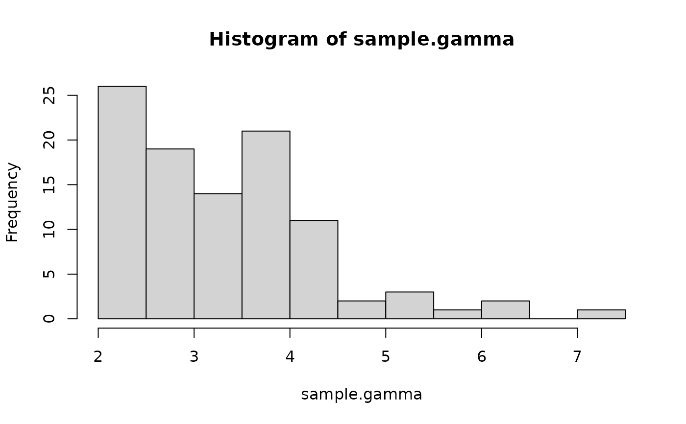
# Gamma distribution
sample.gamma <- rtrunc(n = 100, family = "gamma", shape = 6, rate = 2, a = 2)
hist(sample.gamma, nclass = 15)


# Poisson distribution
sample.pois <- rtrunc(n = 10, family = "poisson", lambda = 10, a = 4)
sample.pois
#>  [1]  8  6  9  7 15  9 14 14  6 11
plot(table(sample.pois))