Probability distributions

In this R lab, we will practice with probability distributions.

Binomial distribution

A random variable $X$ is said to be a binomial variable with parameters $n$ and $p$ if

\[ P(X=x) = \binom n x p^{x}(1-p)^{n-x}\]

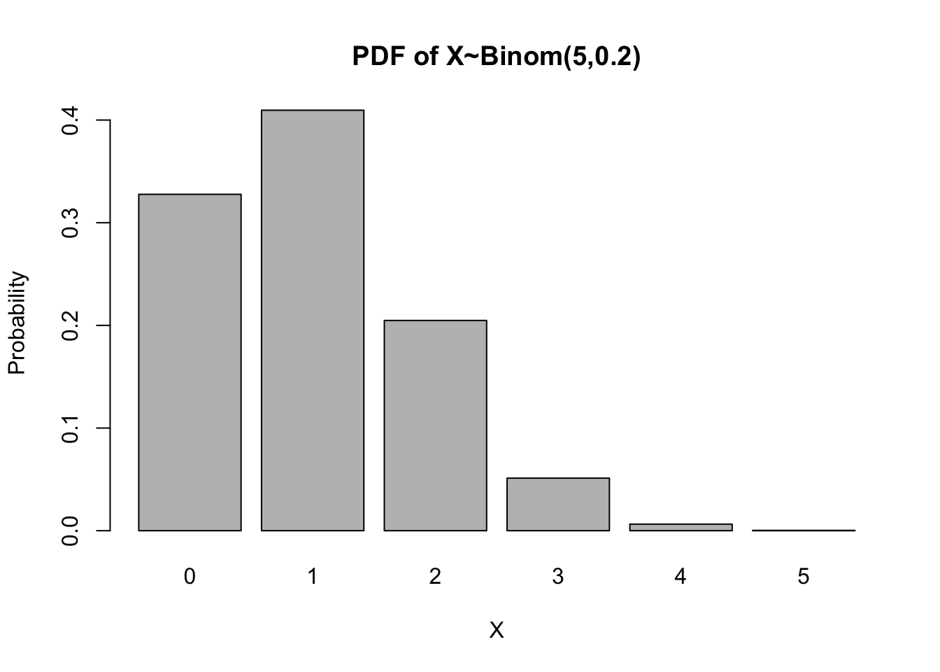
This is often writen $X \sim \text{Binom}(n,p)$. Let us compute the probabilities of a binomial distribution $X \sim \text{Binom}(5,0.2)$ using R.

# first, we store the parameters of the distribution in variables n and p
n = 5
p = 0.2

x = 0:n # we create a vector with discrete values from 0 to n

binom_coef=choose(n, x) # we compute the binomial coefficients for each x 

# we compute binomial probabilities for all x values
binom_prob= binom_coef* p^x * (1 - p)^{n-x} 
print(binom_prob) # we print all probabilities

[1] 0.32768 0.40960 0.20480 0.05120 0.00640 0.00032

This was a good exercise, but R has a built-in function to compute the probabilities of a binomial distribution directly: dbinom(x,n,p). Let us use that function to verify that the probabilities that we computed were correct.

binom_prob = dbinom(x,n,p)
print(binom_prob)

[1] 0.32768 0.40960 0.20480 0.05120 0.00640 0.00032

We can plot those probabilities with the barplot command to see the probability density function (PDF).

barplot(names= x,
        height = binom_prob,
        main = "PDF of X~Binom(5,0.2)",
        xlab='X',
        ylab='Probability')

Simulations of a binomial distribution

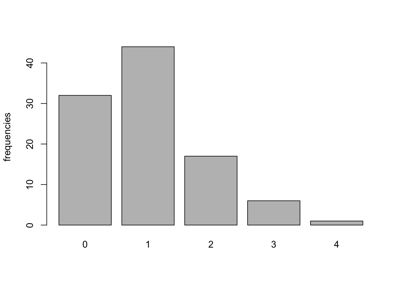
Next we will simulate N samples from a binomial distribution with the command rbinom(N, n, p) and look at the frequency distribution of the outcomes.

N=100
# we draw N samples from a binomial distribution with parameters n and p and store them in variable binom_sim
binom_sim = rbinom(N,n,p)

# we compute the frequency distribution of the samples and store them in a variable
data = table(binom_sim)
print(data)

binom_sim
 0  1  2  3  4 
32 44 17  6  1

# we can plot the frequencies in a bar plot
barplot(data,ylab="frequencies")

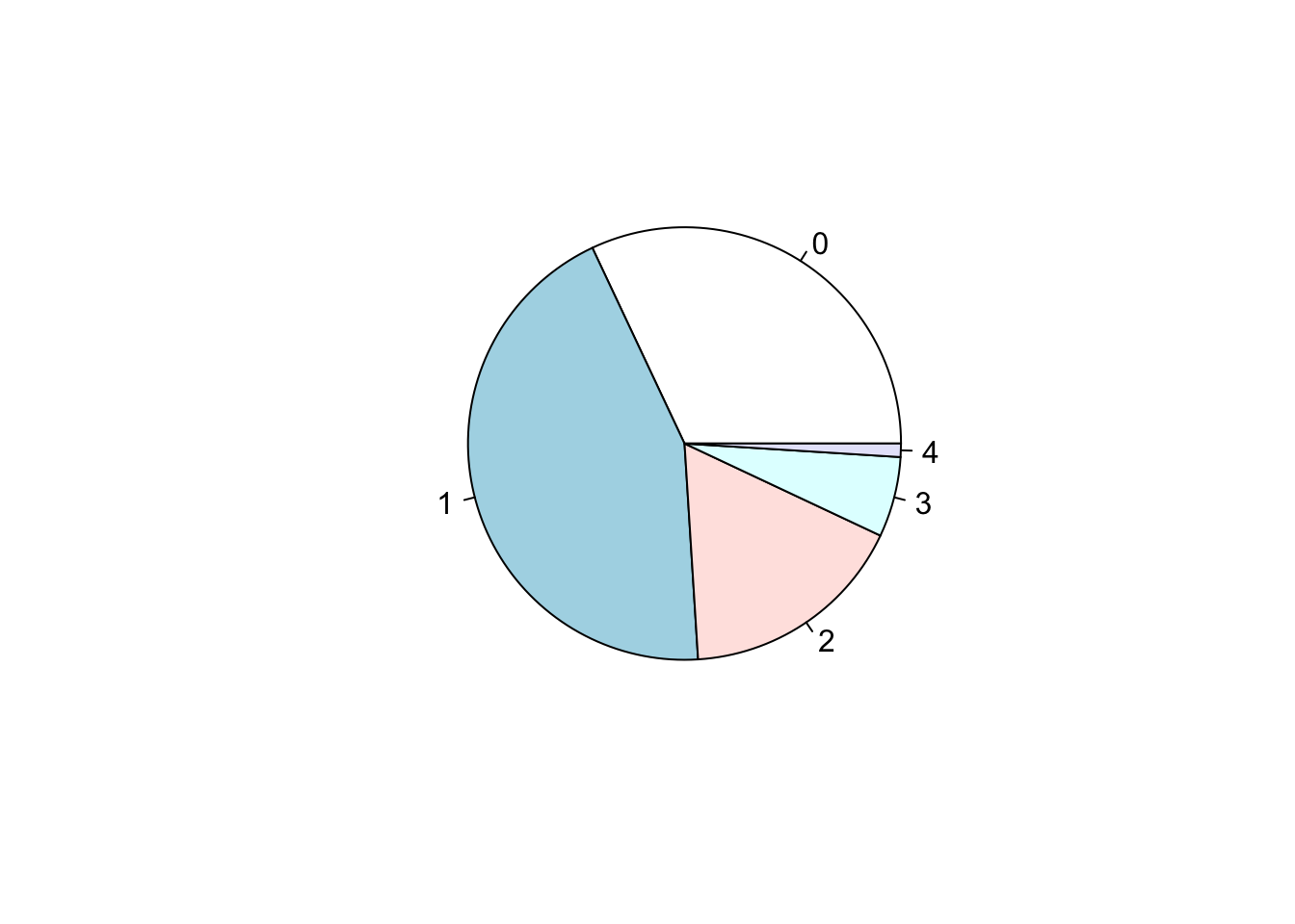
# we can plot the frequencies in a pie chart
pie(data)

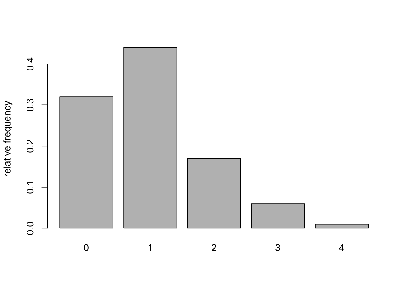
Next, we will compute the relative frequencies by dividing the observed frequencies by the total number of draws N. For high N, the relative frequencies should approach the theoretical probabilities of the binomial distribution.

binom_sim_relfreq=data/N
print(binom_sim_relfreq)

binom_sim
   0    1    2    3    4 
0.32 0.44 0.17 0.06 0.01

barplot(binom_sim_relfreq,ylab="relative frequency")

Normal distribution

The probability density function of the normal distribution $X \sim \text{N}(\mu,\sigma)$, where $\mu$ denotes the mean and $\sigma$ the standard deviation, is given by:

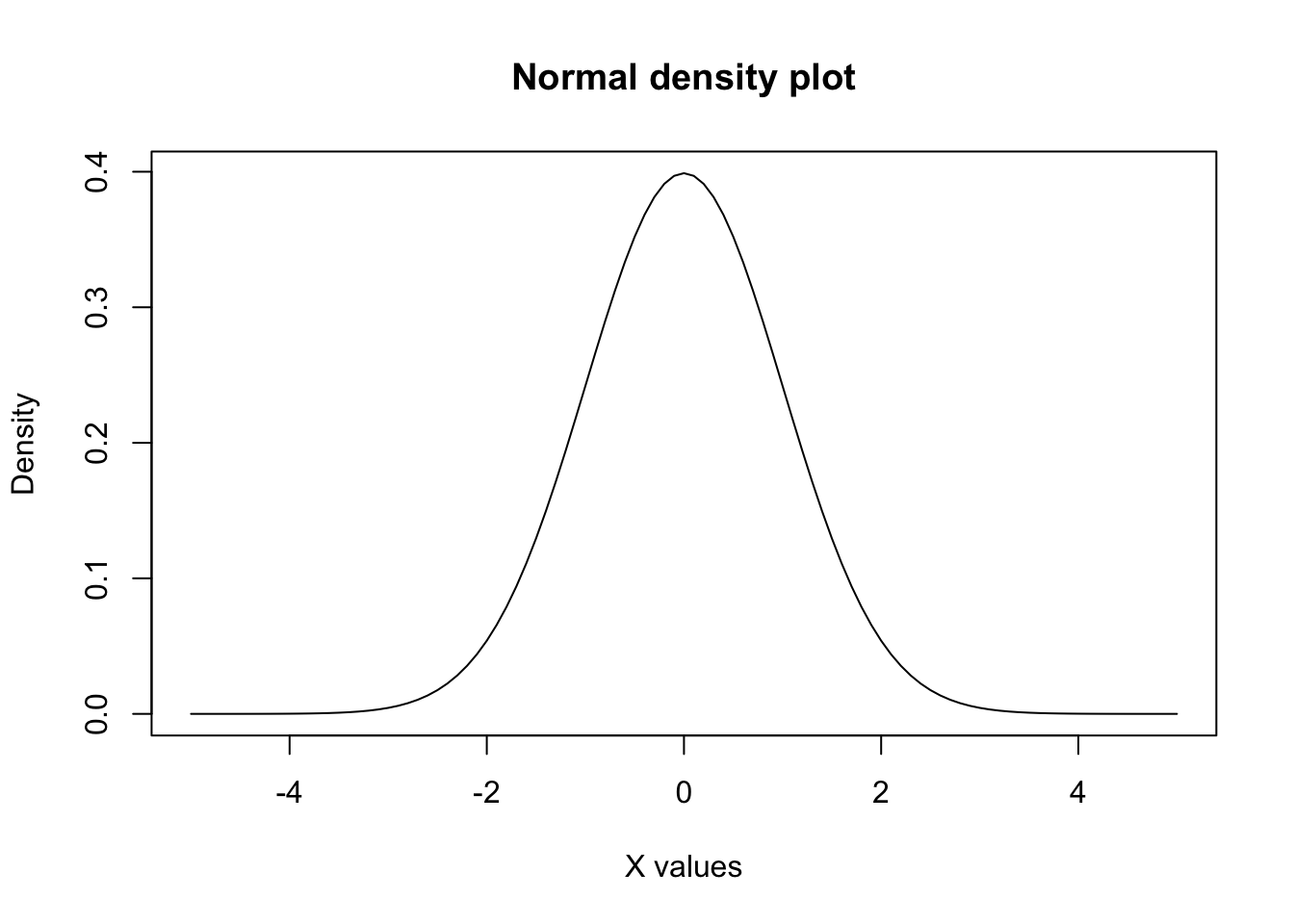
\[ f(x) = \frac{1}{\sigma \sqrt{2\pi}} \text{exp}(- \frac{(x-\mu)^2}{2\sigma^2}) \]

We can define and plot this function in R to see the characteristic bell shape of the normal distribution.

# first we set the values for the mean and the sd 
mu=0
sigma=1

# next, we define the function f
f_norm=function(x){(1/(sigma*sqrt(2*pi))) * exp((-(x-mu)^2)/(2*sigma^2))}
#note that this function is already defined in R as dnorm(x), we could use that instead

# we plot the function f
curve(f_norm,
      xlim=c(-5,5),
      main="Normal density plot",
      xlab="X values",
      ylab="Density"
      )

Next, we will compute $P(X \leq 0)$. For that we can compute the area under the curve from $-\infty$ to $1$ using the function integrate.

integrate(f_norm,-Inf, 0)

0.5 with absolute error < 4.7e-05

Unsurprisingly, R has a built-in function to compute such probabilities: pnorm(x,mean, sd). Let us use that function to verify that the probability that we computed was correct.

pnorm(0, mean=0, sd=1)

[1] 0.5

Conversely, we can find the value of $x$ so that $P(X\leq x) = 0.5$ using the command qnorm(prob,mean,sd).

qnorm(0.5,mean=0,sd=1)

[1] 0

Now let us find the value of $x$ so that $P(-x\leq X\leq x) = 0.95$. As the distribution is symmetric with respect to zero, we could instead find the value of $x$ so that $P( X\leq x) = 0.025$, or equivalently, the value of $x$ so that $P( X\geq x) = 0.025$. We can compute those values again using the command pnorm.

qnorm(0.025,mean=0,sd=1) # find x so that P(X<=x) = 0.025

[1] -1.959964

qnorm(0.025,mean=0,sd=1, lower.tail = FALSE) # find x so that P(X>=x) = 0.025

[1] 1.959964

Let us verify that $P(-1.96\leq X\leq 1.96) = 0.95$.

pnorm(1.96,0,1) - pnorm(-1.96,0,1)

[1] 0.9500042

It is important to remember where the value 1.96 comes from, we will see it later in the course!

Simulations of the normal distribution

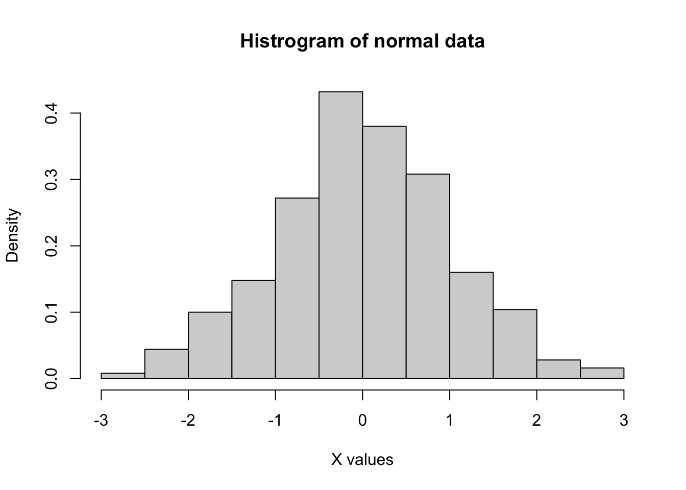
To simulate samples of the normal distribution in R, we use the command rnorm(N, mean, sd). If we want to simulate samples of the standard normal distribution $N(0,1)$, we can simply use the command rnorm(N).

norm_sim=rnorm(500)
hist(norm_sim, 
     freq = FALSE, #This is needed to plot the relative frequencies instead of the frequencies, so that the total area of the histogram is one.
     main= "Histrogram of normal data",
     xlab="X values")

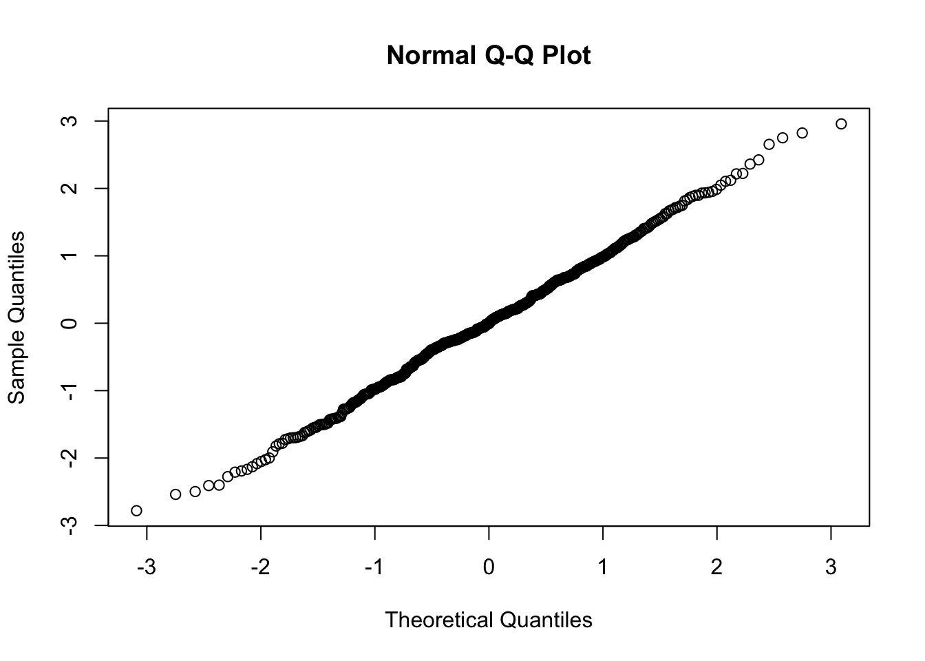
The larger the number of samples, the the closer the histogram would look to a bell shape. We can also check if our data are normally distributed using the command qqnorm(data) that generates a QQPlot. These plots display the data quantiles against the theoretical quantiles of the normal distribution. Therefore, normally distributed data should lie close to the identity line $y=x$.

qqnorm(norm_sim) # we generate the QQPlot for the data simulated data

Approximation of the binomial distribution

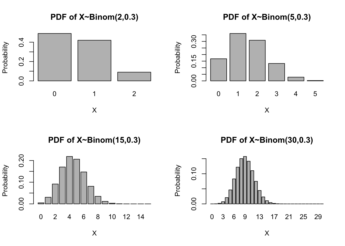
Here we will compute the probability density function of binomial distributions with parameters $p=0.2$ and parameter $n$ variying from 2 to 30.

p=0.3

par(mfrow=c(2,2))    # set the plotting area into a 2*2 matrix
#first plot with n=2
x = 0:2
barplot(names= x,
        height = dbinom(x,2,p),
        main = "PDF of X~Binom(2,0.3)",
        xlab='X',
        ylab='Probability')

#second plot with n=5
x = 0:5
barplot(names= x,
        height = dbinom(x,5,p),
        main = "PDF of X~Binom(5,0.3)",
        xlab='X',
        ylab='Probability')

#third plot with n=15
x = 0:15
barplot(names= x,
        height = dbinom(x,15,p),
        main = "PDF of X~Binom(15,0.3)",
        xlab='X',
        ylab='Probability')

#fourth plot with n=30
x = 0:30
barplot(names= x,
        height = dbinom(x,30,p),
        main = "PDF of X~Binom(30,0.3)",
        xlab='X',
        ylab='Probability')

We observe that the higher $n$ is, the closer the PDF of the binomial distribution looks to a bell shape. From the graphs above, it seems that $X_1 \sim \text{Binom}(30,0.3)$ can be approximated by a normal distribution $X_2 \sim \text{N}(30*0.3,\sqrt{30*0.3*0.7})$. But do the probabilities of anologous events also match? Next, we compare $P(X_1 = 10)$ and $P(9.5 \leq X_2 \leq 10.5)$.

dbinom(x=10,30,0.3)

[1] 0.1415617

mu=30*0.3
sigma=sqrt(30*0.3*0.7) 
pnorm(10.5,mu,sigma) - pnorm(9.5,mu,sigma)

[1] 0.1460026

Exercise: When the normal distribution won’t work

Check if a Binomial distribution with $p=0.01$ and $n=30$ can be approximated by a normal distribution. Why?

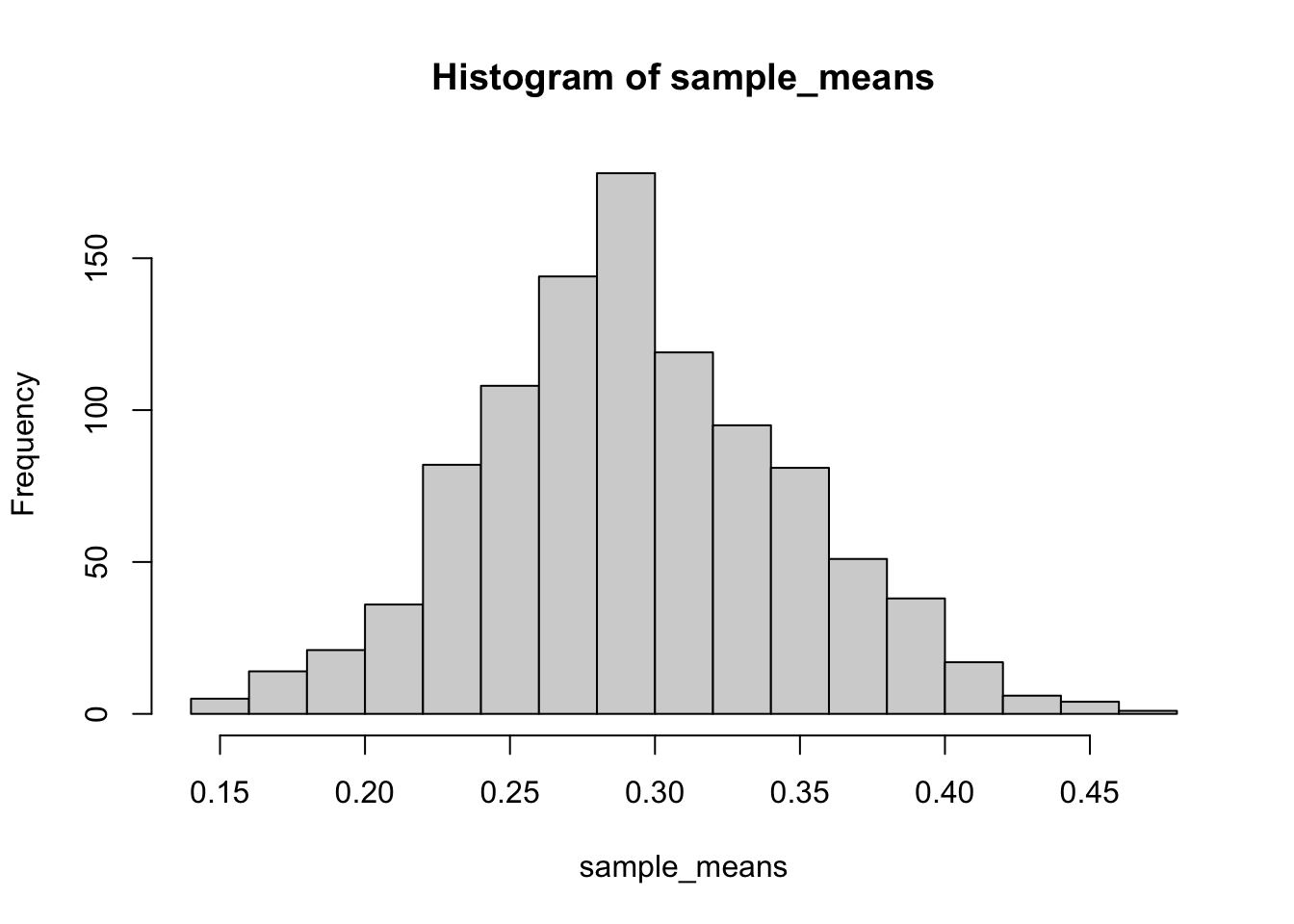
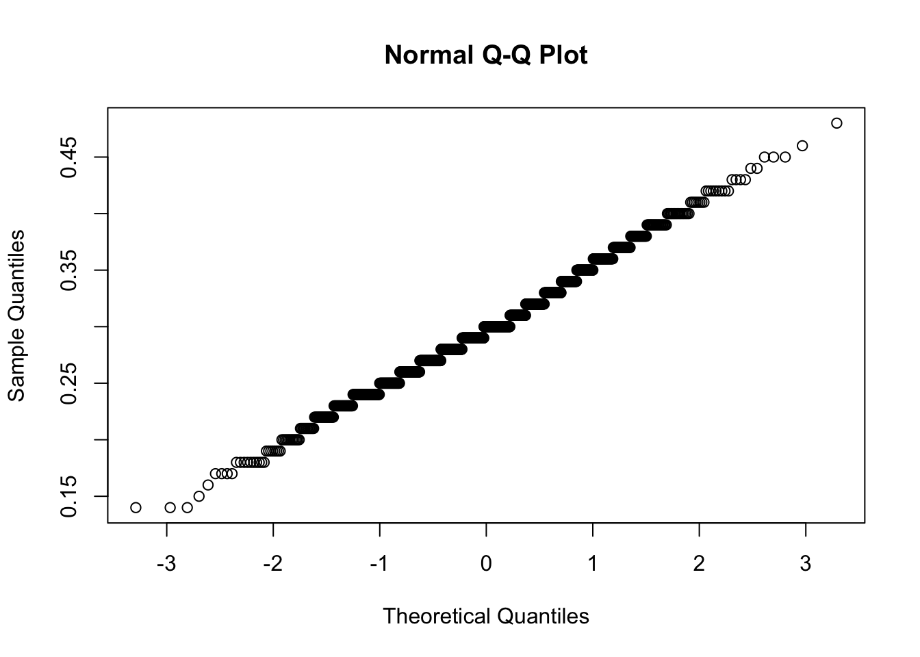
Central Limit Theorem

We will simulate 1000 samples of size $N=100$ of the binomial distribution with parameters $p=0.01$ and $n=30$ (it could be any other distribution). We will compute the mean of each sample and see that the sample mean is a random variable that is normally distributed.

sample_means=replicate(n = 1000, mean(rbinom(100,30,0.01)))
hist(sample_means, breaks=20)

qqnorm(sample_means)

Exercise: Sample mean with small sample size

Repeat the previous simulations, but this time take a very small sample size. Is the sample mean also normally distributed? Why?

--- title: "Probability distributions" format: html: code-fold: false code-tools: true editor: source --- In this R lab, we will practice with probability distributions. ## Binomial distribution A random variable $X$ is said to be a binomial variable with parameters $n$ and $p$ if $$ P(X=x) = \binom n x p^{x}(1-p)^{n-x}$$ This is often writen $X \sim \text{Binom}(n,p)$. Let us compute the probabilities of a binomial distribution $X \sim \text{Binom}(5,0.2)$ using R. ```{r} # first, we store the parameters of the distribution in variables n and p n = 5 p = 0.2 x = 0:n # we create a vector with discrete values from 0 to n binom_coef=choose(n, x) # we compute the binomial coefficients for each x # we compute binomial probabilities for all x values binom_prob= binom_coef* p^x * (1 - p)^{n-x} print(binom_prob) # we print all probabilities ``` This was a good exercise, but R has a built-in function to compute the probabilities of a binomial distribution directly: `dbinom(x,n,p)`. Let us use that function to verify that the probabilities that we computed were correct. ```{r} binom_prob = dbinom(x,n,p) print(binom_prob) ``` We can plot those probabilities with the `barplot` command to see the probability density function (PDF). ```{r} barplot(names= x, height = binom_prob, main = "PDF of X~Binom(5,0.2)", xlab='X', ylab='Probability') ``` ## Simulations of a binomial distribution Next we will simulate N samples from a binomial distribution with the command `rbinom(N, n, p)` and look at the frequency distribution of the outcomes. ```{r} N=100 # we draw N samples from a binomial distribution with parameters n and p and store them in variable binom_sim binom_sim = rbinom(N,n,p) # we compute the frequency distribution of the samples and store them in a variable data = table(binom_sim) print(data) # we can plot the frequencies in a bar plot barplot(data,ylab="frequencies") # we can plot the frequencies in a pie chart pie(data) ``` Next, we will compute the relative frequencies by dividing the observed frequencies by the total number of draws N. For high N, the relative frequencies should approach the theoretical probabilities of the binomial distribution. ```{r} binom_sim_relfreq=data/N print(binom_sim_relfreq) barplot(binom_sim_relfreq,ylab="relative frequency") ``` ## Normal distribution The probability density function of the normal distribution $X \sim \text{N}(\mu,\sigma)$, where $\mu$ denotes the mean and $\sigma$ the standard deviation, is given by: $$ f(x) = \frac{1}{\sigma \sqrt{2\pi}} \text{exp}(- \frac{(x-\mu)^2}{2\sigma^2}) $$ We can define and plot this function in R to see the characteristic bell shape of the normal distribution. ```{r} # first we set the values for the mean and the sd mu=0 sigma=1 # next, we define the function f f_norm=function(x){(1/(sigma*sqrt(2*pi))) * exp((-(x-mu)^2)/(2*sigma^2))} #note that this function is already defined in R as dnorm(x), we could use that instead # we plot the function f curve(f_norm, xlim=c(-5,5), main="Normal density plot", xlab="X values", ylab="Density" ) ``` Next, we will compute $P(X \leq 0)$. For that we can compute the area under the curve from $-\infty$ to $1$ using the function `integrate`. ```{r} integrate(f_norm,-Inf, 0) ``` Unsurprisingly, R has a built-in function to compute such probabilities: `pnorm(x,mean, sd)`. Let us use that function to verify that the probability that we computed was correct. ```{r} pnorm(0, mean=0, sd=1) ``` Conversely, we can find the value of $x$ so that $P(X\leq x) = 0.5$ using the command `qnorm(prob,mean,sd)`. ```{r} qnorm(0.5,mean=0,sd=1) ``` Now let us find the value of $x$ so that $P(-x\leq X\leq x) = 0.95$. As the distribution is symmetric with respect to zero, we could instead find the value of $x$ so that $P( X\leq x) = 0.025$, or equivalently, the value of $x$ so that $P( X\geq x) = 0.025$. We can compute those values again using the command `pnorm`. ```{r} qnorm(0.025,mean=0,sd=1) # find x so that P(X<=x) = 0.025 qnorm(0.025,mean=0,sd=1, lower.tail = FALSE) # find x so that P(X>=x) = 0.025 ``` Let us verify that $P(-1.96\leq X\leq 1.96) = 0.95$. ```{r} pnorm(1.96,0,1) - pnorm(-1.96,0,1) ``` It is important to remember where the value 1.96 comes from, we will see it later in the course! ## Simulations of the normal distribution To simulate samples of the normal distribution in R, we use the command `rnorm(N, mean, sd)`. If we want to simulate samples of the standard normal distribution $N(0,1)$, we can simply use the command `rnorm(N)`. ```{r} norm_sim=rnorm(500) hist(norm_sim, freq = FALSE, #This is needed to plot the relative frequencies instead of the frequencies, so that the total area of the histogram is one. main= "Histrogram of normal data", xlab="X values") ``` The larger the number of samples, the the closer the histogram would look to a bell shape. We can also check if our data are normally distributed using the command `qqnorm(data)` that generates a QQPlot. These plots display the data quantiles against the theoretical quantiles of the normal distribution. Therefore, normally distributed data should lie close to the identity line $y=x$. ```{r} qqnorm(norm_sim) # we generate the QQPlot for the data simulated data ``` ## Approximation of the binomial distribution Here we will compute the probability density function of binomial distributions with parameters $p=0.2$ and parameter $n$ variying from 2 to 30. ```{r} p=0.3 par(mfrow=c(2,2)) # set the plotting area into a 2*2 matrix #first plot with n=2 x = 0:2 barplot(names= x, height = dbinom(x,2,p), main = "PDF of X~Binom(2,0.3)", xlab='X', ylab='Probability') #second plot with n=5 x = 0:5 barplot(names= x, height = dbinom(x,5,p), main = "PDF of X~Binom(5,0.3)", xlab='X', ylab='Probability') #third plot with n=15 x = 0:15 barplot(names= x, height = dbinom(x,15,p), main = "PDF of X~Binom(15,0.3)", xlab='X', ylab='Probability') #fourth plot with n=30 x = 0:30 barplot(names= x, height = dbinom(x,30,p), main = "PDF of X~Binom(30,0.3)", xlab='X', ylab='Probability') ``` We observe that the higher $n$ is, the closer the PDF of the binomial distribution looks to a bell shape. From the graphs above, it seems that $X_1 \sim \text{Binom}(30,0.3)$ can be approximated by a normal distribution $X_2 \sim \text{N}(30*0.3,\sqrt{30*0.3*0.7})$. But do the probabilities of anologous events also match? Next, we compare $P(X_1 = 10)$ and $P(9.5 \leq X_2 \leq 10.5)$. ```{r} dbinom(x=10,30,0.3) mu=30*0.3 sigma=sqrt(30*0.3*0.7) pnorm(10.5,mu,sigma) - pnorm(9.5,mu,sigma) ``` ## Exercise: When the normal distribution won't work Check if a Binomial distribution with $p=0.01$ and $n=30$ can be approximated by a normal distribution. Why? ## Central Limit Theorem We will simulate 1000 samples of size $N=100$ of the binomial distribution with parameters $p=0.01$ and $n=30$ (it could be any other distribution). We will compute the mean of each sample and see that the sample mean is a random variable that is normally distributed. ```{r} sample_means=replicate(n = 1000, mean(rbinom(100,30,0.01))) hist(sample_means, breaks=20) qqnorm(sample_means) ``` ## Exercise: Sample mean with small sample size Repeat the previous simulations, but this time take a very small sample size. Is the sample mean also normally distributed? Why?