R Lab - Part II
Association modeling
In this part of the exercise, we model (on the log-scale) the association of miRNA espression on protein expression adjusting for the corresponding mRNA.
Investigate miR-107 and B-RAF (Aure et al, 2015, Figure 2H)
prt.BRAF = prt[12,]
rna.BRAF = rna[12,]
mir.107 = mir[16,]
(a) Linear regression model
on the log-scale, Aure et al. 2015, equation (3)
fitA <- lm(prt.BRAF ~ mir.107 + rna.BRAF)
summary(fitA)
Call:
lm(formula = prt.BRAF ~ mir.107 + rna.BRAF)

Residuals:
    Min      1Q  Median      3Q     Max
-2.3028 -0.6126  0.0453  0.6153  3.1361

Coefficients:
              Estimate Std. Error t value Pr(>|t|)
(Intercept) -7.315e-08  5.068e-02   0.000        1
mir.107      4.324e-01  5.079e-02   8.513 1.06e-15 ***
rna.BRAF     3.200e-01  5.079e-02   6.301 1.15e-09 ***
---
Signif. codes:  0 '***' 0.001 '**' 0.01 '*' 0.05 '.' 0.1 ' ' 1

Residual standard error: 0.851 on 279 degrees of freedom
Multiple R-squared:  0.281, Adjusted R-squared:  0.2758
F-statistic: 54.51 on 2 and 279 DF,  p-value: < 2.2e-16
Add smooth non-linear cures to the scatterplots: use existing panel.smooth() function, and add linear regression lines to the scatterplots:
panel.linear <- function (x, y, col.regres = "blue", ...)
{
  points(x, y, pch=19)
  ok <- is.finite(x) & is.finite(y)
  if (any(ok))
    abline(stats::lm(y[ok] ~ x[ok]), col = col.regres, ...)
}

pairs(data.frame(mir.107, prt.BRAF, rna.BRAF),
      lower.panel = panel.smooth,
      upper.panel = panel.linear)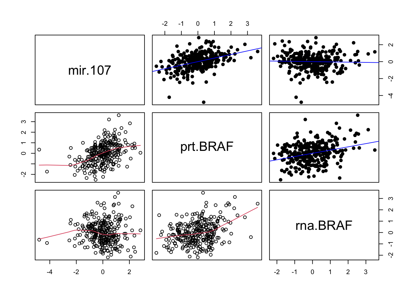
(b) Lasso-penalised linear model
with all miRNAs (Aure et al. 2015, equation (4))
library(glmnet)

# 10-fold CV to determine the optimal lambda:
# Note: rna.BRAF is penalised together with all the mir variables.
# You can use the penalty.factor option to avoid this.
set.seed(1234)
cvfit <- cv.glmnet(y=prt.BRAF, x=t(rbind(mir, rna.BRAF)),
                   alpha=1, nfolds=10, standardize=TRUE)

par(mfrow=c(1,1))
plot(cvfit)
lambda.opt <- cvfit$lambda.min

# Coefficient path plot and coefficients for optimal lambda:
fitB <- cvfit$glmnet.fit

plot(fitB, xvar="lambda")
abline(v=log(lambda.opt))

coef(fitB, s=lambda.opt)
predict(fitB, type="nonzero", s=lambda.opt)
Compare the regression coefficient of mir.107 from the models in (a) and (b):
coef(fitA)["mir.107"]
as.matrix(coef(fitB, s=cvfit$lambda.min))["hsa-miR-107",]
Task 3
Repeat the lasso analysis, but this time do not penalise the rna.BRAF variable together with the mir variables.
Check out the information on the penalty.factor option in ?glmnet to understand how.