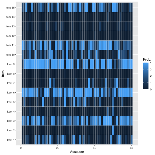
MCMC with Parallel Chains • BayesMallows

library(BayesMallows)
set.seed(123)

This vignette describes how to run Markov chain Monte Carlo with parallel chains. For an introduction to the “BayesMallows” package, please see the introductory vignette, which is an updated version of Sørensen et al. (2020). For parallel processing of particles with the sequential Monte Carlo algorithm of Stein (2023), see the SMC vignette.

Why Parallel Chains?

Modern computers have multiple cores, and on computing clusters one can get access to hundreds of cores easily. By running Markov Chains in parallel on $K$ cores, ideally from different starting points, we achieve at least the following:

The time you have to wait to get the required number of post-burnin samples scales like $1/K$ .
You can check convergence by comparing chains.

Parallel Chains with Complete Rankings

In “BayesMallows” we use the “parallel” package for parallel computation. Parallelization is obtained by starting a cluster and providing it as an argument. Note that we also give one initial value of the dispersion parameter $\alpha$ to each chain.

library(parallel)
cl <- makeCluster(4)
fit <- compute_mallows(
  data = setup_rank_data(rankings = potato_visual), 
  compute_options = set_compute_options(nmc = 5000),
  cl = cl
)
stopCluster(cl)

We can assess convergence in the usual way:

assess_convergence(fit)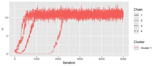

Trace plot of scale parameter for four chains.

We can also assess convergence for the latent ranks $\boldsymbol{\rho}$ . Since the initial value of $\boldsymbol{\rho}$ is sampled uniformly, the two chains automatically get different initial values.

assess_convergence(fit, parameter = "rho", items = 1:3)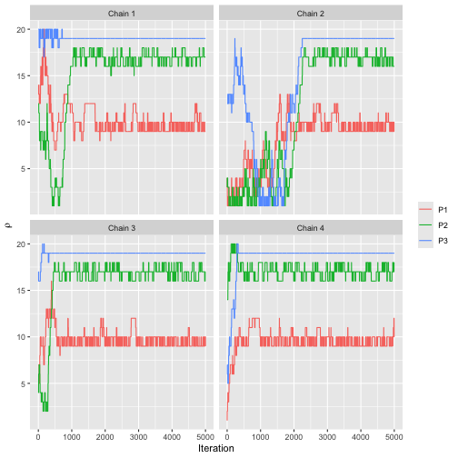

Trace plot of modal ranking for four chains.

Based on the convergence plots, we set the burnin to 3000.

burnin(fit) <- 3000

We can now use all the tools for assessing the posterior distributions as usual. The post-burnin samples for all parallel chains are simply combined, as they should be.

Below is a plot of the posterior distribution of $\alpha$ .

plot(fit)

Posterior of scale parameter, combing post-burnin samples from all chains.

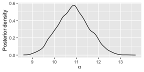
Next is a plot of the posterior distribution of $\boldsymbol{\rho}$ .

plot(fit, parameter = "rho", items = 4:7)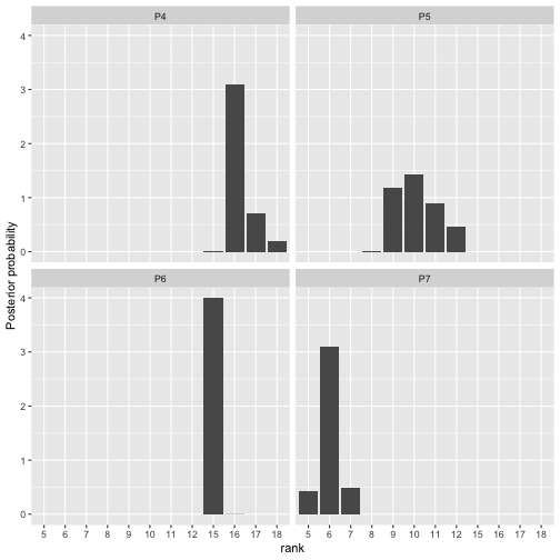

Posterior of modal ranking, combing post-burnin samples from all chains.

Parallel Chains with Pairwise Preferences

A case where parallel chains might be more strongly needed is with incomplete data, e.g., arising from pairwise preferences. In this case the MCMC algorithm needs to perform data augmentation, which tends to be both slow and sticky. We illustrate this with the beach preference data, again referring to Sørensen et al. (2020) for a more thorough introduction to the aspects not directly related to parallelism.

beach_data <- setup_rank_data(preferences = beach_preferences)

We run four parallel chains, letting the package generate random initial rankings, but again providing a vector of initial values for $\alpha$ .

cl <- makeCluster(4)
fit <- compute_mallows(
  data = beach_data,
  compute_options = set_compute_options(nmc = 4000, save_aug = TRUE),
  initial_values = set_initial_values(alpha_init = runif(4, 1, 4)),
  cl = cl
)
stopCluster(cl)

Trace Plots

The convergence plots shows some long-range autocorrelation, but otherwise it seems to mix relatively well.

assess_convergence(fit)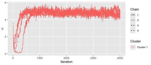

Trace plot of scale parameter for beach preferences data, on four chains.

Here is the convergence plot for $\boldsymbol{\rho}$ :

assess_convergence(fit, parameter = "rho", items = 4:6)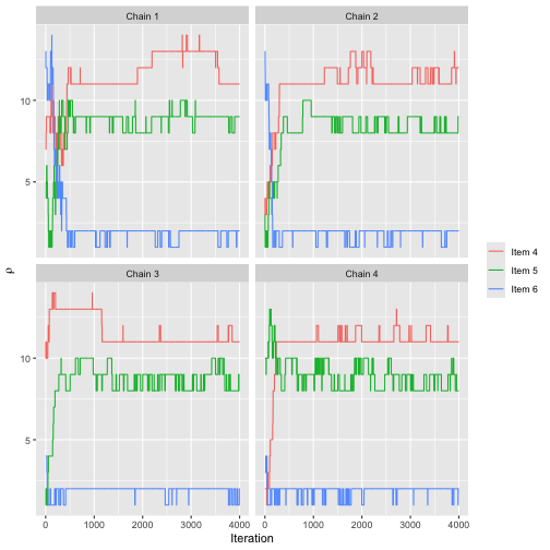

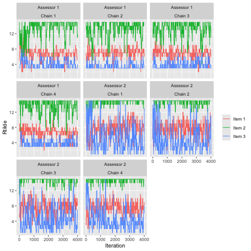
Trace plot of modal ranking for beach preferences data, on four chains.

To avoid overplotting, it’s a good idea to pick a low number of assessors and chains. We here look at items 1-3 of assessors 1 and 2.

assess_convergence(fit,
  parameter = "Rtilde",
  items = 1:3, assessors = 1:2
)

Trace plot of augmented rankings for beach preference data, on four chains.

Posterior Quantities

Based on the trace plots, the chains seem to be mixing well. We set the burnin to 1000.

burnin(fit) <- 1000

We can now study the posterior distributions. Here is the posterior for $\alpha$ . Note that by increasing the nmc argument to compute_mallows above, the density would appear smoother. In this vignette we have kept it low to reduce the run time.

plot(fit)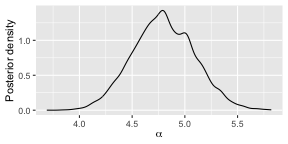

Posterior distribution for scale parameter.

We can also look at the posterior for $\boldsymbol{\rho}$ .

plot(fit, parameter = "rho", items = 6:9)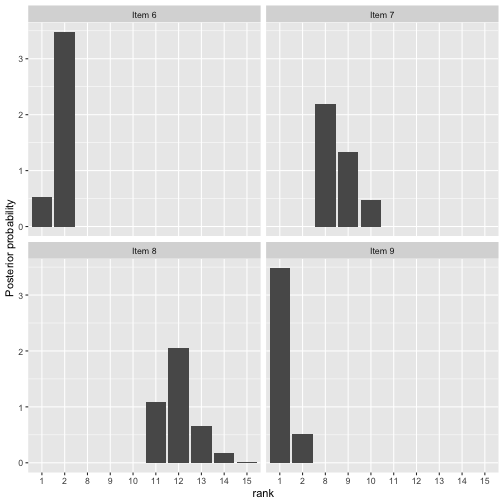

Posterior distribution for modal rankings.

We can also compute posterior intervals in the usual way:

compute_posterior_intervals(fit, parameter = "alpha")
#>   parameter  mean median          hpdi central_interval
#> 1     alpha 4.798  4.793 [4.242,5.373]    [4.235,5.371]

compute_posterior_intervals(fit, parameter = "rho")
#>    parameter    item mean median    hpdi central_interval
#> 1        rho  Item 1    7      7     [7]            [6,7]
#> 2        rho  Item 2   15     15    [15]          [14,15]
#> 3        rho  Item 3    3      3   [3,4]            [3,4]
#> 4        rho  Item 4   11     11 [11,13]          [11,13]
#> 5        rho  Item 5    9      9  [8,10]           [8,10]
#> 6        rho  Item 6    2      2   [1,2]            [1,2]
#> 7        rho  Item 7    9      8  [8,10]           [8,10]
#> 8        rho  Item 8   12     12 [11,13]          [11,14]
#> 9        rho  Item 9    1      1   [1,2]            [1,2]
#> 10       rho Item 10    6      6   [5,6]            [5,7]
#> 11       rho Item 11    4      4   [3,5]            [3,5]
#> 12       rho Item 12   13     13 [12,14]          [11,14]
#> 13       rho Item 13   10     10  [8,10]           [8,10]
#> 14       rho Item 14   13     14 [12,14]          [12,14]
#> 15       rho Item 15    5      5   [4,5]            [4,6]

And we can compute the consensus ranking:

compute_consensus(fit)
#>      cluster ranking    item   cumprob
#> 1  Cluster 1       1  Item 9 0.8691667
#> 2  Cluster 1       2  Item 6 1.0000000
#> 3  Cluster 1       3  Item 3 0.6391667
#> 4  Cluster 1       4 Item 11 0.9404167
#> 5  Cluster 1       5 Item 15 0.9559167
#> 6  Cluster 1       6 Item 10 0.9636667
#> 7  Cluster 1       7  Item 1 1.0000000
#> 8  Cluster 1       8  Item 7 0.5473333
#> 9  Cluster 1       9  Item 5 0.9255833
#> 10 Cluster 1      10 Item 13 1.0000000
#> 11 Cluster 1      11  Item 4 0.6924167
#> 12 Cluster 1      12  Item 8 0.7833333
#> 13 Cluster 1      13 Item 12 0.6158333
#> 14 Cluster 1      14 Item 14 0.9958333
#> 15 Cluster 1      15  Item 2 1.0000000

compute_consensus(fit, type = "MAP")
#>      cluster map_ranking    item probability
#> 1  Cluster 1           1  Item 9   0.2683333
#> 2  Cluster 1           2  Item 6   0.2683333
#> 3  Cluster 1           3  Item 3   0.2683333
#> 4  Cluster 1           4 Item 11   0.2683333
#> 5  Cluster 1           5 Item 15   0.2683333
#> 6  Cluster 1           6 Item 10   0.2683333
#> 7  Cluster 1           7  Item 1   0.2683333
#> 8  Cluster 1           8  Item 7   0.2683333
#> 9  Cluster 1           9  Item 5   0.2683333
#> 10 Cluster 1          10 Item 13   0.2683333
#> 11 Cluster 1          11  Item 4   0.2683333
#> 12 Cluster 1          12  Item 8   0.2683333
#> 13 Cluster 1          13 Item 12   0.2683333
#> 14 Cluster 1          14 Item 14   0.2683333
#> 15 Cluster 1          15  Item 2   0.2683333

We can compute the probability of being top- $k$ , here for $k=4$ :

plot_top_k(fit, k = 4)

Probability of being top-4 for beach preference data.

References

Sørensen, Øystein, Marta Crispino, Qinghua Liu, and Valeria Vitelli. 2020. “BayesMallows: An R Package for the Bayesian Mallows Model.” The R Journal 12 (1): 324–42. https://doi.org/10.32614/RJ-2020-026.

Stein, Anja. 2023. “Sequential Inference with the Mallows Model.” PhD thesis, Lancaster University.