Preference Learning with the Mallows Rank Model

Compute the posterior distributions of the parameters of the Bayesian Mallows Rank Model, given rankings or preferences stated by a set of assessors.

The BayesMallows package uses the following parametrization of the Mallows rank model (Mallows 1957) :

$$p(r|\alpha,\rho) = \frac{1}{Z_{n}(\alpha)} \exp\left\{\frac{-\alpha}{n} d(r,\rho)\right\}$$

where $r$ is a ranking, $\alpha$ is a scale parameter, $\rho$ is the latent consensus ranking, $Z_{n}(\alpha)$ is the partition function (normalizing constant), and $d(r,\rho)$ is a distance function measuring the distance between $r$ and $\rho$. We refer to Vitelli et al. (2018) for further details of the Bayesian Mallows model.

compute_mallows always returns posterior distributions of the latent consensus ranking $\rho$ and the scale parameter $\alpha$. Several distance measures are supported, and the preferences can take the form of complete or incomplete rankings, as well as pairwise preferences. compute_mallows can also compute mixtures of Mallows models, for clustering of assessors with similar preferences.

Usage

compute_mallows(
  data,
  model_options = set_model_options(),
  compute_options = set_compute_options(),
  priors = set_priors(),
  initial_values = set_initial_values(),
  pfun_estimate = NULL,
  progress_report = set_progress_report(),
  cl = NULL
)

Arguments

data: An object of class "BayesMallowsData" returned from setup_rank_data().
model_options: An object of class "BayesMallowsModelOptions" returned from set_model_options().
compute_options: An object of class "BayesMallowsComputeOptions" returned from set_compute_options().
priors: An object of class "BayesMallowsPriors" returned from set_priors().
initial_values: An object of class "BayesMallowsInitialValues" returned from set_initial_values().
pfun_estimate: Object returned from estimate_partition_function(). Defaults to NULL, and will only be used for footrule, Spearman, or Ulam distances when the cardinalities are not available, cf. get_cardinalities().
progress_report: An object of class "BayesMallowsProgressReported" returned from set_progress_report().
cl: Optional cluster returned from parallel::makeCluster(). If provided, chains will be run in parallel, one on each node of cl.

Value

An object of class BayesMallows.

References

Mallows CL (1957). “Non-Null Ranking Models. I.” Biometrika, 44(1/2), 114–130.

Vitelli V, Sørensen, Crispino M, Arjas E, Frigessi A (2018). “Probabilistic Preference Learning with the Mallows Rank Model.” Journal of Machine Learning Research, 18(1), 1–49. https://jmlr.org/papers/v18/15-481.html.

Examples

# ANALYSIS OF COMPLETE RANKINGS
# The example datasets potato_visual and potato_weighing contain complete
# rankings of 20 items, by 12 assessors. We first analyse these using the Mallows
# model:
set.seed(1)
model_fit <- compute_mallows(
  data = setup_rank_data(rankings = potato_visual),
  compute_options = set_compute_options(nmc = 2000)
  )

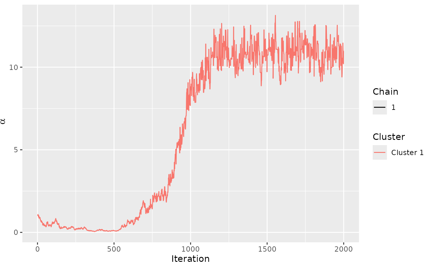
# We study the trace plot of the parameters
assess_convergence(model_fit, parameter = "alpha")

assess_convergence(model_fit, parameter = "rho", items = 1:4)


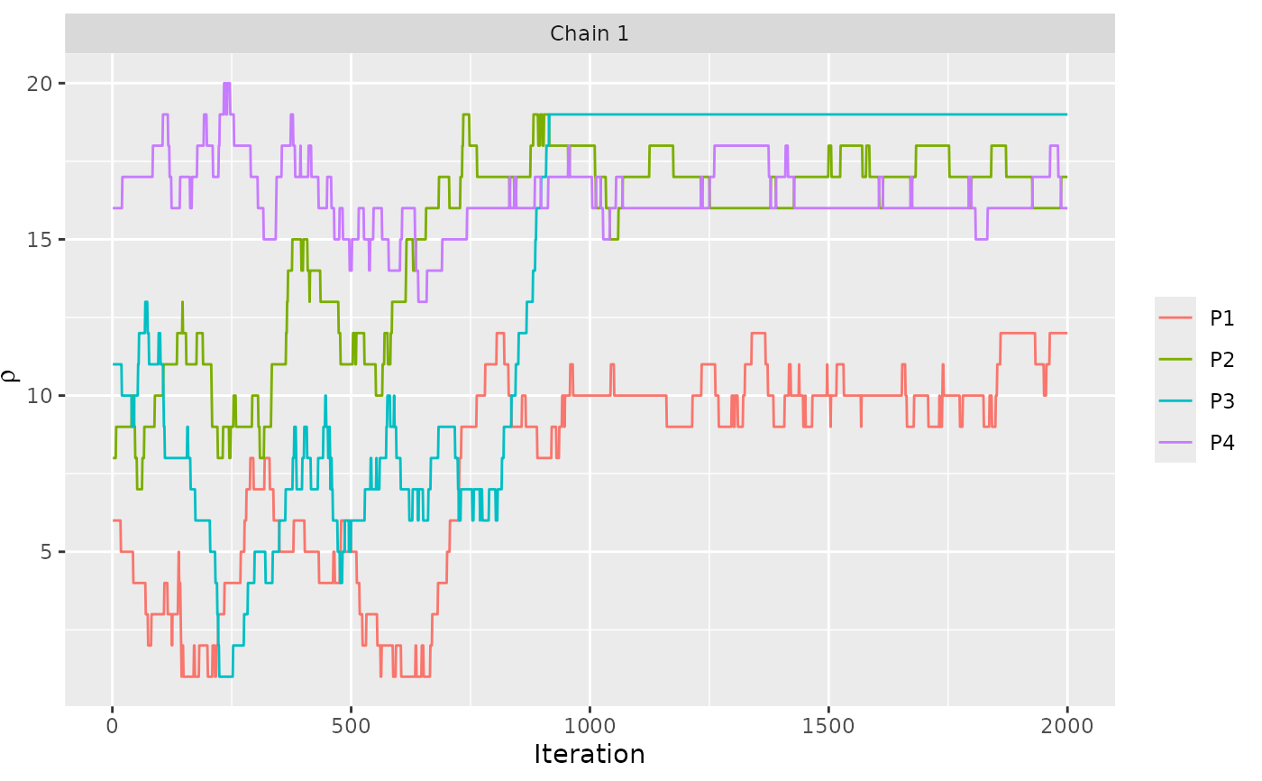# Based on these plots, we set burnin = 1000.
burnin(model_fit) <- 1000
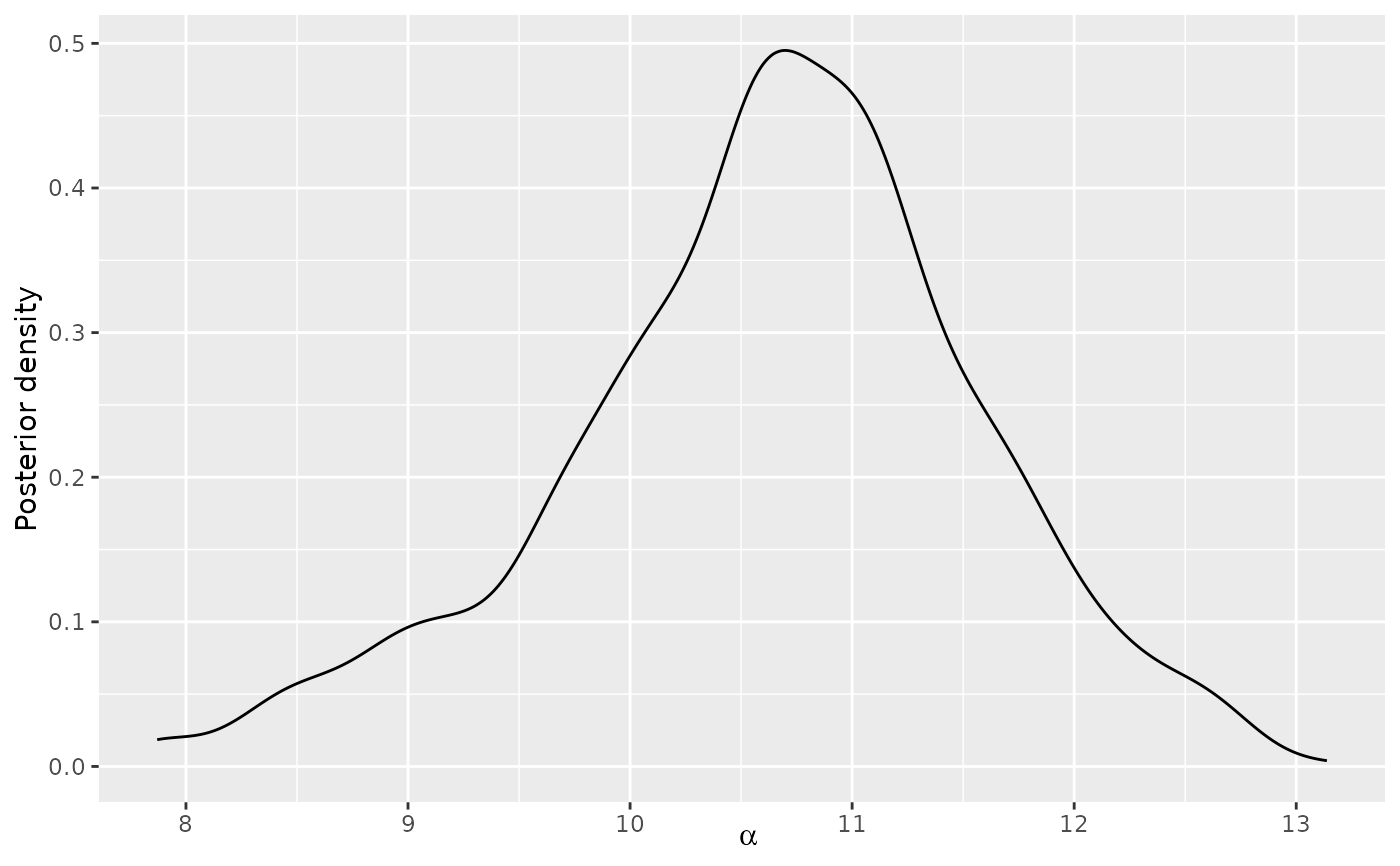
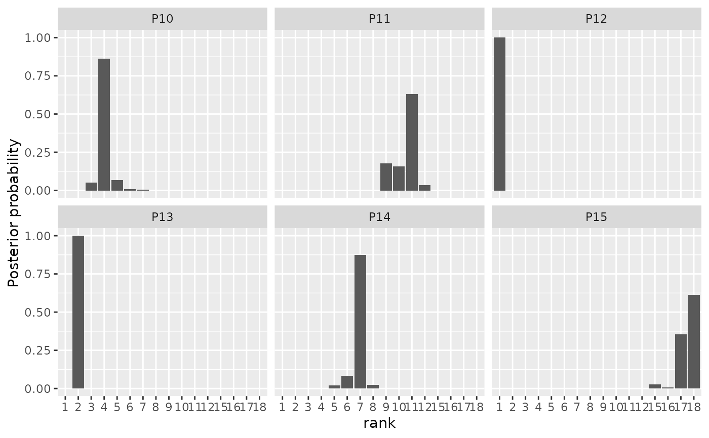
# Next, we use the generic plot function to study the posterior distributions
# of alpha and rho
plot(model_fit, parameter = "alpha")

plot(model_fit, parameter = "rho", items = 10:15)


# We can also compute the CP consensus posterior ranking
compute_consensus(model_fit, type = "CP")
#>      cluster ranking item cumprob
#> 1  Cluster 1       1  P12   1.000
#> 2  Cluster 1       2  P13   1.000
#> 3  Cluster 1       3   P9   0.876
#> 4  Cluster 1       4  P10   0.916
#> 5  Cluster 1       5  P17   0.748
#> 6  Cluster 1       6   P7   0.882
#> 7  Cluster 1       7  P14   0.977
#> 8  Cluster 1       8  P16   0.845
#> 9  Cluster 1       9   P5   0.605
#> 10 Cluster 1      10   P1   0.743
#> 11 Cluster 1      11  P11   0.965
#> 12 Cluster 1      12  P19   1.000
#> 13 Cluster 1      13  P20   0.582
#> 14 Cluster 1      14  P18   1.000
#> 15 Cluster 1      15   P6   0.916
#> 16 Cluster 1      16   P4   0.727
#> 17 Cluster 1      17   P2   0.780
#> 18 Cluster 1      18  P15   1.000
#> 19 Cluster 1      19   P3   1.000
#> 20 Cluster 1      20   P8   1.000

# And we can compute the posterior intervals:
# First we compute the interval for alpha
compute_posterior_intervals(model_fit, parameter = "alpha")
#>   parameter   mean median           hpdi central_interval
#> 1     alpha 10.632 10.704 [8.468,12.259]   [8.473,12.352]
# Then we compute the interval for all the items
compute_posterior_intervals(model_fit, parameter = "rho")
#>    parameter item mean median      hpdi central_interval
#> 1        rho   P1   10     10    [9,12]           [9,12]
#> 2        rho   P2   17     17   [16,18]          [16,18]
#> 3        rho   P3   19     19      [19]             [19]
#> 4        rho   P4   16     16   [16,18]          [15,18]
#> 5        rho   P5    9      9 [3][6,11]           [3,11]
#> 6        rho   P6   15     15   [15,16]          [15,18]
#> 7        rho   P7    6      6     [5,7]            [5,7]
#> 8        rho   P8   20     20      [20]             [20]
#> 9        rho   P9    3      3     [3,4]            [3,4]
#> 10       rho  P10    4      4     [3,5]            [3,5]
#> 11       rho  P11   11     11    [9,11]           [9,12]
#> 12       rho  P12    1      1       [1]              [1]
#> 13       rho  P13    2      2       [2]              [2]
#> 14       rho  P14    7      7     [6,7]            [6,7]
#> 15       rho  P15   18     18   [17,18]          [15,18]
#> 16       rho  P16    8      8     [8,9]            [8,9]
#> 17       rho  P17    5      5  [5,6][8]            [5,8]
#> 18       rho  P18   14     14   [13,14]          [13,14]
#> 19       rho  P19   12     12  [10][12]          [10,12]
#> 20       rho  P20   13     13   [13,14]          [13,14]

# ANALYSIS OF PAIRWISE PREFERENCES
# The example dataset beach_preferences contains pairwise
# preferences between beaches stated by 60 assessors. There
# is a total of 15 beaches in the dataset.
beach_data <- setup_rank_data(
  preferences = beach_preferences
)
# We then run the Bayesian Mallows rank model
# We save the augmented data for diagnostics purposes.
model_fit <- compute_mallows(
  data = beach_data,
  compute_options = set_compute_options(save_aug = TRUE),
  progress_report = set_progress_report(verbose = TRUE))
#> First 1000 iterations of Metropolis-Hastings algorithm completed.
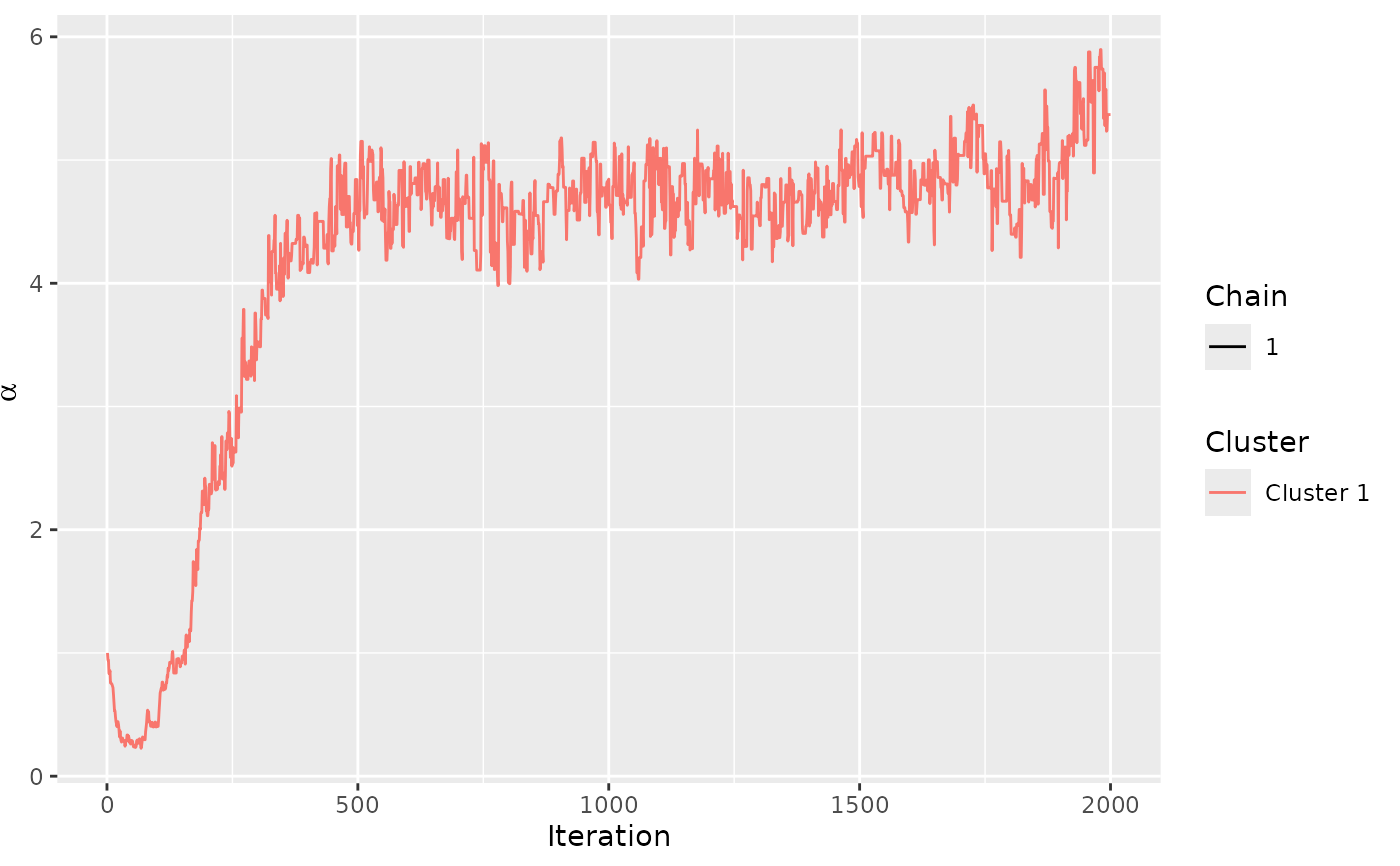
# We can assess the convergence of the scale parameter
assess_convergence(model_fit)

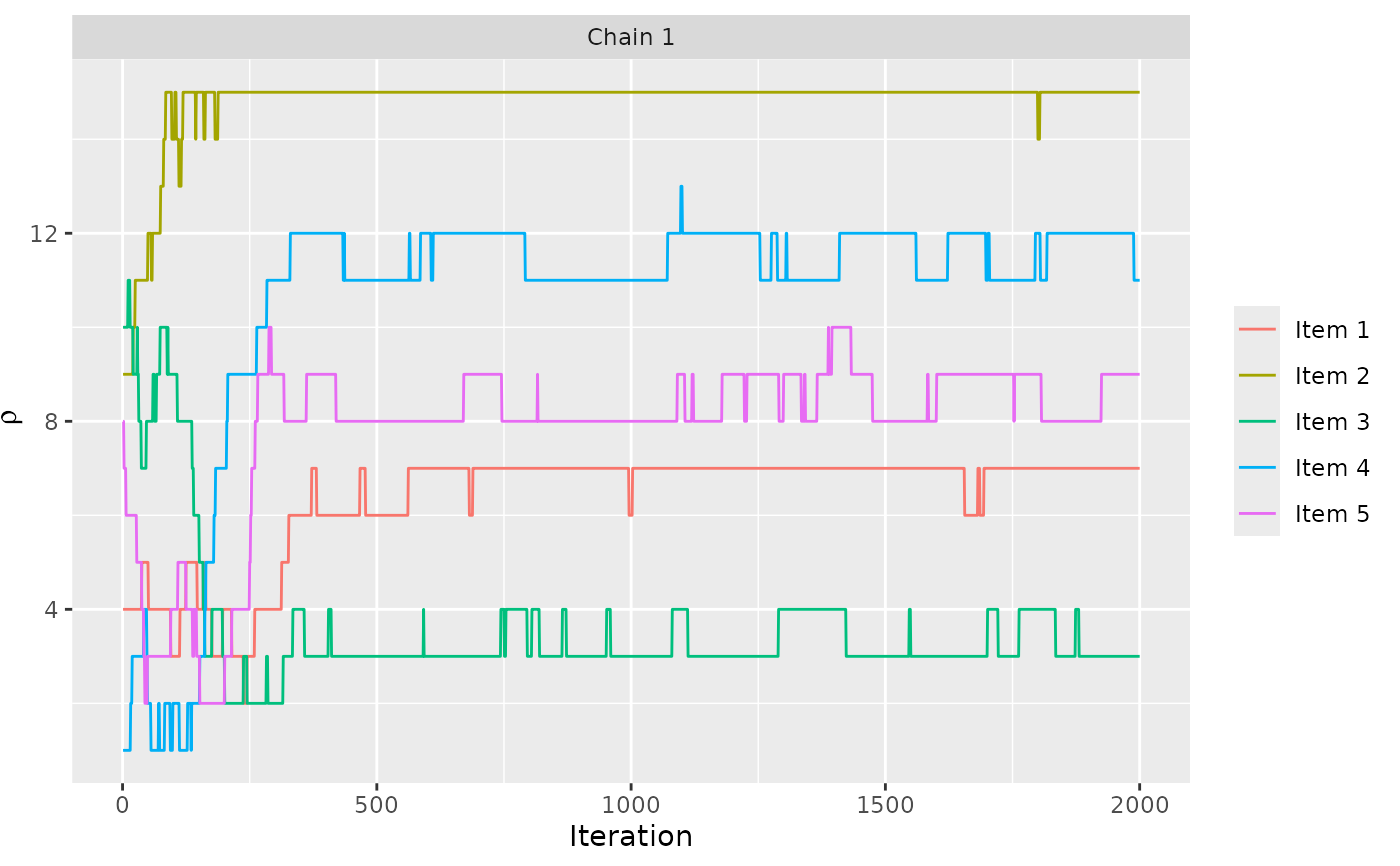
# We can assess the convergence of latent rankings. Here we
# show beaches 1-5.
assess_convergence(model_fit, parameter = "rho", items = 1:5)

# We can also look at the convergence of the augmented rankings for
# each assessor.
assess_convergence(model_fit, parameter = "Rtilde",
                   items = c(2, 4), assessors = c(1, 2))

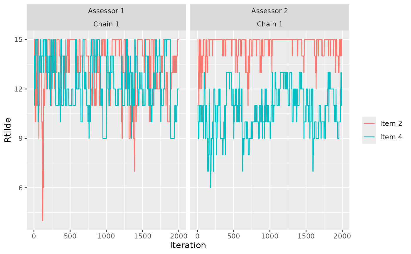# Notice how, for assessor 1, the lines cross each other, while
# beach 2 consistently has a higher rank value (lower preference) for
# assessor 2. We can see why by looking at the implied orderings in
# beach_tc
subset(get_transitive_closure(beach_data), assessor %in% c(1, 2) &
         bottom_item %in% c(2, 4) & top_item %in% c(2, 4))
#>    assessor bottom_item top_item
#> 49        2           2        4
# Assessor 1 has no implied ordering between beach 2 and beach 4,
# while assessor 2 has the implied ordering that beach 4 is preferred
# to beach 2. This is reflected in the trace plots.


# CLUSTERING OF ASSESSORS WITH SIMILAR PREFERENCES
if (FALSE) { # \dontrun{
  # The example dataset sushi_rankings contains 5000 complete
  # rankings of 10 types of sushi
  # We start with computing a 3-cluster solution
  model_fit <- compute_mallows(
    data = setup_rank_data(sushi_rankings),
    model_options = set_model_options(n_clusters = 3),
    compute_options = set_compute_options(nmc = 10000),
    progress_report = set_progress_report(verbose = TRUE))
  # We then assess convergence of the scale parameter alpha
  assess_convergence(model_fit)
  # Next, we assess convergence of the cluster probabilities
  assess_convergence(model_fit, parameter = "cluster_probs")
  # Based on this, we set burnin = 1000
  # We now plot the posterior density of the scale parameters alpha in
  # each mixture:
  burnin(model_fit) <- 1000
  plot(model_fit, parameter = "alpha")
  # We can also compute the posterior density of the cluster probabilities
  plot(model_fit, parameter = "cluster_probs")
  # We can also plot the posterior cluster assignment. In this case,
  # the assessors are sorted according to their maximum a posteriori cluster estimate.
  plot(model_fit, parameter = "cluster_assignment")
  # We can also assign each assessor to a cluster
  cluster_assignments <- assign_cluster(model_fit, soft = FALSE)
  } # }

# DETERMINING THE NUMBER OF CLUSTERS
if (FALSE) { # \dontrun{
  # Continuing with the sushi data, we can determine the number of cluster
  # Let us look at any number of clusters from 1 to 10
  # We use the convenience function compute_mallows_mixtures
  n_clusters <- seq(from = 1, to = 10)
  models <- compute_mallows_mixtures(
    n_clusters = n_clusters,
    data = setup_rank_data(rankings = sushi_rankings),
    compute_options = set_compute_options(
      nmc = 6000, alpha_jump = 10, include_wcd = TRUE)
    )
  # models is a list in which each element is an object of class BayesMallows,
  # returned from compute_mallows
  # We can create an elbow plot
  burnin(models) <- 1000
  plot_elbow(models)
  # We then select the number of cluster at a point where this plot has
  # an "elbow", e.g., at 6 clusters.
} # }

# SPEEDING UP COMPUTION WITH OBSERVATION FREQUENCIES With a large number of
# assessors taking on a relatively low number of unique rankings, the
# observation_frequency argument allows providing a rankings matrix with the
# unique set of rankings, and the observation_frequency vector giving the number
# of assessors with each ranking. This is illustrated here for the potato_visual
# dataset
#
# assume each row of potato_visual corresponds to between 1 and 5 assessors, as
# given by the observation_frequency vector
if (FALSE) { # \dontrun{
  set.seed(1234)
  observation_frequency <- sample.int(n = 5, size = nrow(potato_visual), replace = TRUE)
  m <- compute_mallows(
    setup_rank_data(rankings = potato_visual, observation_frequency = observation_frequency))

  # INTRANSITIVE PAIRWISE PREFERENCES
  set.seed(1234)
  mod <- compute_mallows(
    setup_rank_data(preferences = bernoulli_data),
    compute_options = set_compute_options(nmc = 5000),
    priors = set_priors(kappa = c(1, 10)),
    model_options = set_model_options(error_model = "bernoulli")
  )

  assess_convergence(mod)
  assess_convergence(mod, parameter = "theta")
  burnin(mod) <- 3000

  plot(mod)
  plot(mod, parameter = "theta")
} # }
# CHEKING FOR LABEL SWITCHING
if (FALSE) { # \dontrun{
  # This example shows how to assess if label switching happens in BayesMallows
  # We start by creating a directory in which csv files with individual
  # cluster probabilities should be saved in each step of the MCMC algorithm
  # NOTE: For computational efficiency, we use much fewer MCMC iterations than one
  # would normally do.
  dir.create("./test_label_switch")
  # Next, we go into this directory
  setwd("./test_label_switch/")
  # For comparison, we run compute_mallows with and without saving the cluster
  # probabilities The purpose of this is to assess the time it takes to save
  # the cluster probabilites.
  system.time(m <- compute_mallows(
    setup_rank_data(rankings = sushi_rankings),
    model_options = set_model_options(n_clusters = 3),
    compute_options = set_compute_options(nmc = 500, save_ind_clus = FALSE)))
  # With this options, compute_mallows will save cluster_probs2.csv,
  # cluster_probs3.csv, ..., cluster_probs[nmc].csv.
  system.time(m <- compute_mallows(
    setup_rank_data(rankings = sushi_rankings),
    model_options = set_model_options(n_clusters = 3),
    compute_options = set_compute_options(nmc = 500, save_ind_clus = TRUE)))

  # Next, we check convergence of alpha
  assess_convergence(m)

  # We set the burnin to 200
  burnin <- 200

  # Find all files that were saved. Note that the first file saved is
  # cluster_probs2.csv
  cluster_files <- list.files(pattern = "cluster\\_probs[[:digit:]]+\\.csv")

  # Check the size of the files that were saved.
  paste(sum(do.call(file.size, list(cluster_files))) * 1e-6, "MB")

  # Find the iteration each file corresponds to, by extracting its number
  iteration_number <- as.integer(
    regmatches(x = cluster_files,m = regexpr(pattern = "[0-9]+", cluster_files)
               ))
  # Remove all files before burnin
  file.remove(cluster_files[iteration_number <= burnin])
  # Update the vector of files, after the deletion
  cluster_files <- list.files(pattern = "cluster\\_probs[[:digit:]]+\\.csv")
  # Create 3d array, with dimensions (iterations, assessors, clusters)
  prob_array <- array(
    dim = c(length(cluster_files), m$data$n_assessors, m$n_clusters))
  # Read each file, adding to the right element of the array
  for(i in seq_along(cluster_files)){
    prob_array[i, , ] <- as.matrix(
      read.csv(cluster_files[[i]], header = FALSE))
  }

  # Create an integer array of latent allocations, as this is required by
  # label.switching
  z <- subset(m$cluster_assignment, iteration > burnin)
  z$value <- as.integer(gsub("Cluster ", "", z$value))
  z$chain <- NULL
  z <- reshape(z, direction = "wide", idvar = "iteration", timevar = "assessor")
  z$iteration <- NULL
  z <- as.matrix(z)

  # Now apply Stephen's algorithm
  library(label.switching)
  switch_check <- label.switching("STEPHENS", z = z,
                                  K = m$n_clusters, p = prob_array)

  # Check the proportion of cluster assignments that were switched
  mean(apply(switch_check$permutations$STEPHENS, 1, function(x) {
    !all(x == seq(1, m$n_clusters, by = 1))
  }))

  # Remove the rest of the csv files
  file.remove(cluster_files)
  # Move up one directory
  setwd("..")
  # Remove the directory in which the csv files were saved
  file.remove("./test_label_switch/")
} # }

Usage

Arguments

Value

References

See also

Examples