Example: Single experiment

In the R package, we’ve attached two example datasets from a large drug combination screening experiment on diffuse large B-cell lymphoma. We’ll use these to show some simple use cases of the main functions and how to interpret the results.

Let’s load in the first example and have a look at it

library(bayesynergy)
data("mathews_DLBCL")
y = mathews_DLBCL[[1]][[1]]
x = mathews_DLBCL[[1]][[2]]
head(cbind(y,x))

##      Viability ibrutinib ispinesib
## [1,] 1.2295618    0.0000         0
## [2,] 1.0376006    0.1954         0
## [3,] 1.1813851    0.7812         0
## [4,] 0.5882688    3.1250         0
## [5,] 0.4666700   12.5000         0
## [6,] 0.2869514   50.0000         0

We see that the the measured viability scores are stored in the vector y, while x is a matrix with two columns giving the corresponding concentrations where the viability scores were read off.

Fitting the regression model is simple enough, and can be done on default settings simply by running the following code (where we add the names of the drugs involved, the concentration units for plotting purposes, and calculate the bayes factor).

fit = bayesynergy(y,x, drug_names = c("ibrutinib", "ispinesib"),
                  units = c("nM","nM"),bayes_factor = T)

## 
## SAMPLING FOR MODEL 'gp_grid' NOW (CHAIN 1).
## Chain 1: 
## Chain 1: Gradient evaluation took 7.7e-05 seconds
## Chain 1: 1000 transitions using 10 leapfrog steps per transition would take 0.77 seconds.
## Chain 1: Adjust your expectations accordingly!
## Chain 1: 
## Chain 1: 
## Chain 1: Iteration:    1 / 2000 [  0%]  (Warmup)
## Chain 1: Iteration:  200 / 2000 [ 10%]  (Warmup)
## Chain 1: Iteration:  400 / 2000 [ 20%]  (Warmup)
## Chain 1: Iteration:  600 / 2000 [ 30%]  (Warmup)
## Chain 1: Iteration:  800 / 2000 [ 40%]  (Warmup)
## Chain 1: Iteration: 1000 / 2000 [ 50%]  (Warmup)
## Chain 1: Iteration: 1001 / 2000 [ 50%]  (Sampling)
## Chain 1: Iteration: 1200 / 2000 [ 60%]  (Sampling)
## Chain 1: Iteration: 1400 / 2000 [ 70%]  (Sampling)
## Chain 1: Iteration: 1600 / 2000 [ 80%]  (Sampling)
## Chain 1: Iteration: 1800 / 2000 [ 90%]  (Sampling)
## Chain 1: Iteration: 2000 / 2000 [100%]  (Sampling)
## Chain 1: 
## Chain 1:  Elapsed Time: 2.653 seconds (Warm-up)
## Chain 1:                2.437 seconds (Sampling)
## Chain 1:                5.09 seconds (Total)
## Chain 1: 
## 
## SAMPLING FOR MODEL 'gp_grid' NOW (CHAIN 2).
## Chain 2: 
## Chain 2: Gradient evaluation took 6.3e-05 seconds
## Chain 2: 1000 transitions using 10 leapfrog steps per transition would take 0.63 seconds.
## Chain 2: Adjust your expectations accordingly!
## Chain 2: 
## Chain 2: 
## Chain 2: Iteration:    1 / 2000 [  0%]  (Warmup)
## Chain 2: Iteration:  200 / 2000 [ 10%]  (Warmup)
## Chain 2: Iteration:  400 / 2000 [ 20%]  (Warmup)
## Chain 2: Iteration:  600 / 2000 [ 30%]  (Warmup)
## Chain 2: Iteration:  800 / 2000 [ 40%]  (Warmup)
## Chain 2: Iteration: 1000 / 2000 [ 50%]  (Warmup)
## Chain 2: Iteration: 1001 / 2000 [ 50%]  (Sampling)
## Chain 2: Iteration: 1200 / 2000 [ 60%]  (Sampling)
## Chain 2: Iteration: 1400 / 2000 [ 70%]  (Sampling)
## Chain 2: Iteration: 1600 / 2000 [ 80%]  (Sampling)
## Chain 2: Iteration: 1800 / 2000 [ 90%]  (Sampling)
## Chain 2: Iteration: 2000 / 2000 [100%]  (Sampling)
## Chain 2: 
## Chain 2:  Elapsed Time: 2.646 seconds (Warm-up)
## Chain 2:                4.777 seconds (Sampling)
## Chain 2:                7.423 seconds (Total)
## Chain 2: 
## 
## SAMPLING FOR MODEL 'gp_grid' NOW (CHAIN 3).
## Chain 3: 
## Chain 3: Gradient evaluation took 4.7e-05 seconds
## Chain 3: 1000 transitions using 10 leapfrog steps per transition would take 0.47 seconds.
## Chain 3: Adjust your expectations accordingly!
## Chain 3: 
## Chain 3: 
## Chain 3: Iteration:    1 / 2000 [  0%]  (Warmup)
## Chain 3: Iteration:  200 / 2000 [ 10%]  (Warmup)
## Chain 3: Iteration:  400 / 2000 [ 20%]  (Warmup)
## Chain 3: Iteration:  600 / 2000 [ 30%]  (Warmup)
## Chain 3: Iteration:  800 / 2000 [ 40%]  (Warmup)
## Chain 3: Iteration: 1000 / 2000 [ 50%]  (Warmup)
## Chain 3: Iteration: 1001 / 2000 [ 50%]  (Sampling)
## Chain 3: Iteration: 1200 / 2000 [ 60%]  (Sampling)
## Chain 3: Iteration: 1400 / 2000 [ 70%]  (Sampling)
## Chain 3: Iteration: 1600 / 2000 [ 80%]  (Sampling)
## Chain 3: Iteration: 1800 / 2000 [ 90%]  (Sampling)
## Chain 3: Iteration: 2000 / 2000 [100%]  (Sampling)
## Chain 3: 
## Chain 3:  Elapsed Time: 2.183 seconds (Warm-up)
## Chain 3:                2.437 seconds (Sampling)
## Chain 3:                4.62 seconds (Total)
## Chain 3: 
## 
## SAMPLING FOR MODEL 'gp_grid' NOW (CHAIN 4).
## Chain 4: 
## Chain 4: Gradient evaluation took 4.6e-05 seconds
## Chain 4: 1000 transitions using 10 leapfrog steps per transition would take 0.46 seconds.
## Chain 4: Adjust your expectations accordingly!
## Chain 4: 
## Chain 4: 
## Chain 4: Iteration:    1 / 2000 [  0%]  (Warmup)
## Chain 4: Iteration:  200 / 2000 [ 10%]  (Warmup)
## Chain 4: Iteration:  400 / 2000 [ 20%]  (Warmup)
## Chain 4: Iteration:  600 / 2000 [ 30%]  (Warmup)
## Chain 4: Iteration:  800 / 2000 [ 40%]  (Warmup)
## Chain 4: Iteration: 1000 / 2000 [ 50%]  (Warmup)
## Chain 4: Iteration: 1001 / 2000 [ 50%]  (Sampling)
## Chain 4: Iteration: 1200 / 2000 [ 60%]  (Sampling)
## Chain 4: Iteration: 1400 / 2000 [ 70%]  (Sampling)
## Chain 4: Iteration: 1600 / 2000 [ 80%]  (Sampling)
## Chain 4: Iteration: 1800 / 2000 [ 90%]  (Sampling)
## Chain 4: Iteration: 2000 / 2000 [100%]  (Sampling)
## Chain 4: 
## Chain 4:  Elapsed Time: 2.141 seconds (Warm-up)
## Chain 4:                2.034 seconds (Sampling)
## Chain 4:                4.175 seconds (Total)
## Chain 4: 
## 
## SAMPLING FOR MODEL 'nointeraction' NOW (CHAIN 1).
## Chain 1: 
## Chain 1: Gradient evaluation took 2.5e-05 seconds
## Chain 1: 1000 transitions using 10 leapfrog steps per transition would take 0.25 seconds.
## Chain 1: Adjust your expectations accordingly!
## Chain 1: 
## Chain 1: 
## Chain 1: Iteration:    1 / 2000 [  0%]  (Warmup)
## Chain 1: Iteration:  200 / 2000 [ 10%]  (Warmup)
## Chain 1: Iteration:  400 / 2000 [ 20%]  (Warmup)
## Chain 1: Iteration:  600 / 2000 [ 30%]  (Warmup)
## Chain 1: Iteration:  800 / 2000 [ 40%]  (Warmup)
## Chain 1: Iteration: 1000 / 2000 [ 50%]  (Warmup)
## Chain 1: Iteration: 1001 / 2000 [ 50%]  (Sampling)
## Chain 1: Iteration: 1200 / 2000 [ 60%]  (Sampling)
## Chain 1: Iteration: 1400 / 2000 [ 70%]  (Sampling)
## Chain 1: Iteration: 1600 / 2000 [ 80%]  (Sampling)
## Chain 1: Iteration: 1800 / 2000 [ 90%]  (Sampling)
## Chain 1: Iteration: 2000 / 2000 [100%]  (Sampling)
## Chain 1: 
## Chain 1:  Elapsed Time: 0.33 seconds (Warm-up)
## Chain 1:                0.356 seconds (Sampling)
## Chain 1:                0.686 seconds (Total)
## Chain 1: 
## 
## SAMPLING FOR MODEL 'nointeraction' NOW (CHAIN 2).
## Chain 2: 
## Chain 2: Gradient evaluation took 1.8e-05 seconds
## Chain 2: 1000 transitions using 10 leapfrog steps per transition would take 0.18 seconds.
## Chain 2: Adjust your expectations accordingly!
## Chain 2: 
## Chain 2: 
## Chain 2: Iteration:    1 / 2000 [  0%]  (Warmup)
## Chain 2: Iteration:  200 / 2000 [ 10%]  (Warmup)
## Chain 2: Iteration:  400 / 2000 [ 20%]  (Warmup)
## Chain 2: Iteration:  600 / 2000 [ 30%]  (Warmup)
## Chain 2: Iteration:  800 / 2000 [ 40%]  (Warmup)
## Chain 2: Iteration: 1000 / 2000 [ 50%]  (Warmup)
## Chain 2: Iteration: 1001 / 2000 [ 50%]  (Sampling)
## Chain 2: Iteration: 1200 / 2000 [ 60%]  (Sampling)
## Chain 2: Iteration: 1400 / 2000 [ 70%]  (Sampling)
## Chain 2: Iteration: 1600 / 2000 [ 80%]  (Sampling)
## Chain 2: Iteration: 1800 / 2000 [ 90%]  (Sampling)
## Chain 2: Iteration: 2000 / 2000 [100%]  (Sampling)
## Chain 2: 
## Chain 2:  Elapsed Time: 0.358 seconds (Warm-up)
## Chain 2:                0.203 seconds (Sampling)
## Chain 2:                0.561 seconds (Total)
## Chain 2: 
## 
## SAMPLING FOR MODEL 'nointeraction' NOW (CHAIN 3).
## Chain 3: 
## Chain 3: Gradient evaluation took 1.7e-05 seconds
## Chain 3: 1000 transitions using 10 leapfrog steps per transition would take 0.17 seconds.
## Chain 3: Adjust your expectations accordingly!
## Chain 3: 
## Chain 3: 
## Chain 3: Iteration:    1 / 2000 [  0%]  (Warmup)
## Chain 3: Iteration:  200 / 2000 [ 10%]  (Warmup)
## Chain 3: Iteration:  400 / 2000 [ 20%]  (Warmup)
## Chain 3: Iteration:  600 / 2000 [ 30%]  (Warmup)
## Chain 3: Iteration:  800 / 2000 [ 40%]  (Warmup)
## Chain 3: Iteration: 1000 / 2000 [ 50%]  (Warmup)
## Chain 3: Iteration: 1001 / 2000 [ 50%]  (Sampling)
## Chain 3: Iteration: 1200 / 2000 [ 60%]  (Sampling)
## Chain 3: Iteration: 1400 / 2000 [ 70%]  (Sampling)
## Chain 3: Iteration: 1600 / 2000 [ 80%]  (Sampling)
## Chain 3: Iteration: 1800 / 2000 [ 90%]  (Sampling)
## Chain 3: Iteration: 2000 / 2000 [100%]  (Sampling)
## Chain 3: 
## Chain 3:  Elapsed Time: 0.342 seconds (Warm-up)
## Chain 3:                0.331 seconds (Sampling)
## Chain 3:                0.673 seconds (Total)
## Chain 3: 
## 
## SAMPLING FOR MODEL 'nointeraction' NOW (CHAIN 4).
## Chain 4: 
## Chain 4: Gradient evaluation took 1.8e-05 seconds
## Chain 4: 1000 transitions using 10 leapfrog steps per transition would take 0.18 seconds.
## Chain 4: Adjust your expectations accordingly!
## Chain 4: 
## Chain 4: 
## Chain 4: Iteration:    1 / 2000 [  0%]  (Warmup)
## Chain 4: Iteration:  200 / 2000 [ 10%]  (Warmup)
## Chain 4: Iteration:  400 / 2000 [ 20%]  (Warmup)
## Chain 4: Iteration:  600 / 2000 [ 30%]  (Warmup)
## Chain 4: Iteration:  800 / 2000 [ 40%]  (Warmup)
## Chain 4: Iteration: 1000 / 2000 [ 50%]  (Warmup)
## Chain 4: Iteration: 1001 / 2000 [ 50%]  (Sampling)
## Chain 4: Iteration: 1200 / 2000 [ 60%]  (Sampling)
## Chain 4: Iteration: 1400 / 2000 [ 70%]  (Sampling)
## Chain 4: Iteration: 1600 / 2000 [ 80%]  (Sampling)
## Chain 4: Iteration: 1800 / 2000 [ 90%]  (Sampling)
## Chain 4: Iteration: 2000 / 2000 [100%]  (Sampling)
## Chain 4: 
## Chain 4:  Elapsed Time: 0.354 seconds (Warm-up)
## Chain 4:                0.358 seconds (Sampling)
## Chain 4:                0.712 seconds (Total)
## Chain 4:

## Calculating the Bayes factor

The resulting model can be summarised by running

summary(fit)

##                 mean  se_mean     sd      2.5%       50%  97.5% n_eff  Rhat
## la_1[1]       0.3301 0.002757 0.0782  1.29e-01  3.44e-01  0.453   804 1.005
## la_2[1]       0.3866 0.002824 0.0652  1.40e-01  3.97e-01  0.458   533 1.008
## log10_ec50_1  0.4866 0.005445 0.1636  2.48e-01  4.48e-01  0.908   902 1.004
## log10_ec50_2 -1.0332 0.019955 1.0356 -3.41e+00 -8.69e-01  0.491  2693 1.000
## slope_1       2.0305 0.020574 0.9436  8.39e-01  1.82e+00  4.462  2103 1.002
## slope_2       1.4765 0.017784 1.0723  1.05e-01  1.22e+00  4.218  3636 1.001
## ell           3.0663 0.034693 1.5244  1.24e+00  2.71e+00  6.958  1931 1.002
## sigma_f       0.8416 0.017847 0.8069  1.70e-01  6.09e-01  2.830  2044 1.002
## s             0.0969 0.000275 0.0149  7.30e-02  9.52e-02  0.131  2956 1.000
## dss_1        33.5129 0.043268 2.8622  2.76e+01  3.36e+01 39.018  4376 1.000
## dss_2        59.4368 0.042907 2.8725  5.36e+01  5.95e+01 64.731  4482 1.000
## rVUS_f       82.7751 0.013496 0.8629  8.11e+01  8.28e+01 84.453  4088 1.000
## rVUS_p0      73.0558 0.031947 2.2230  6.85e+01  7.31e+01 77.257  4842 0.999
## VUS_Delta    -9.7193 0.034040 2.3820 -1.46e+01 -9.65e+00 -5.295  4897 1.000
## VUS_syn      -9.7633 0.033685 2.3422 -1.46e+01 -9.68e+00 -5.490  4835 1.000
## VUS_ant       0.0440 0.001873 0.1079  5.45e-06  8.02e-05  0.372  3318 1.000
## 
## log-Pseudo Marginal Likelihood (LPML) =  50.9839 
## Estimated Bayes factor in favor of full model over non-interaction only model:  34.16251

which gives posterior summaries of the parameters of the model.

In addition, the model calculates summary statistics of the monotherapy curves and the dose-response surface including drug sensitivity scores (DSS) for the two drugs in question, as well as the volumes that capture the notion of efficacy (rVUS_f), interaction (VUS_Delta), synergy (VUS_syn) and interaction (VUS_ant).

As indicated, the total combined drug efficacy is around 80% (rVUS_f), of which around 70 percentage points can be attributed to $p_0$ (rVUS_p0), leaving room for 10 percentage points worth of synergy (VUS_syn). We can also note that the model is fairly certain of this effect, with a 95% credible interval given as (-14.618, -5.49). The certainty of this is also verified by the Bayes factor, which at 34.16 indicates strong evidence of an interaction effect present in the model.

Visualization

Monotherapy curves, 2D contour plots

We can also create plots by simply running

plot(fit, plot3D = F)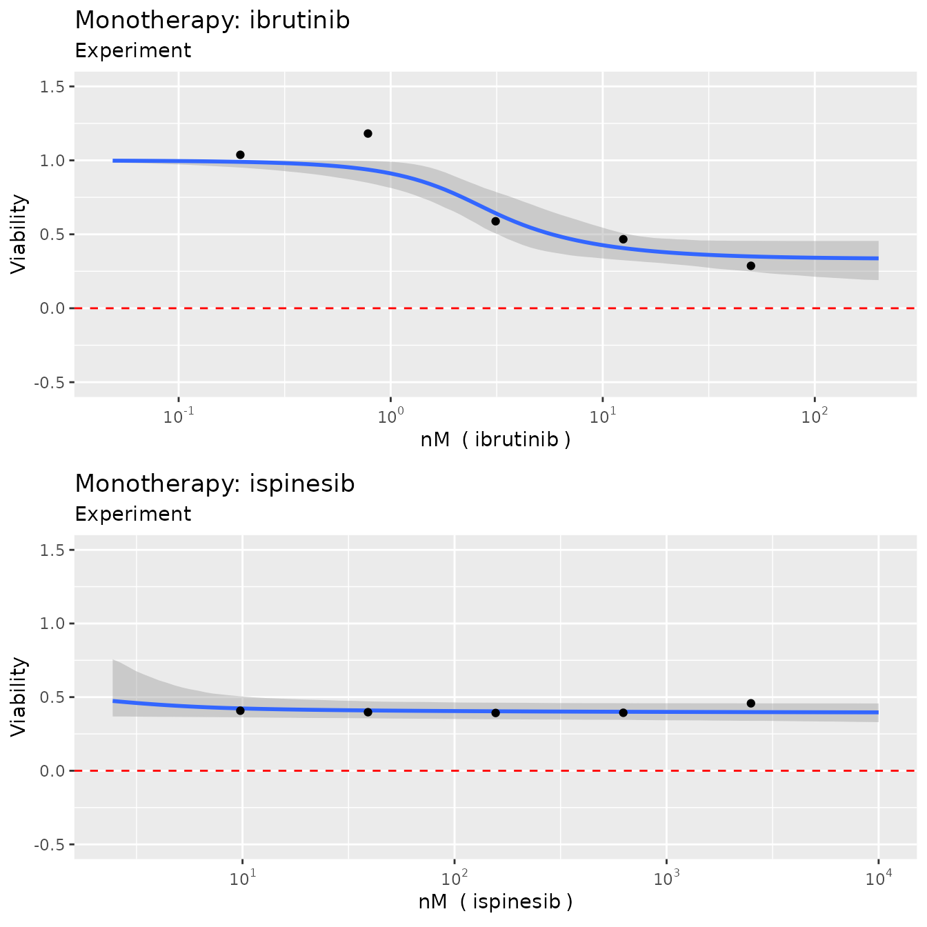

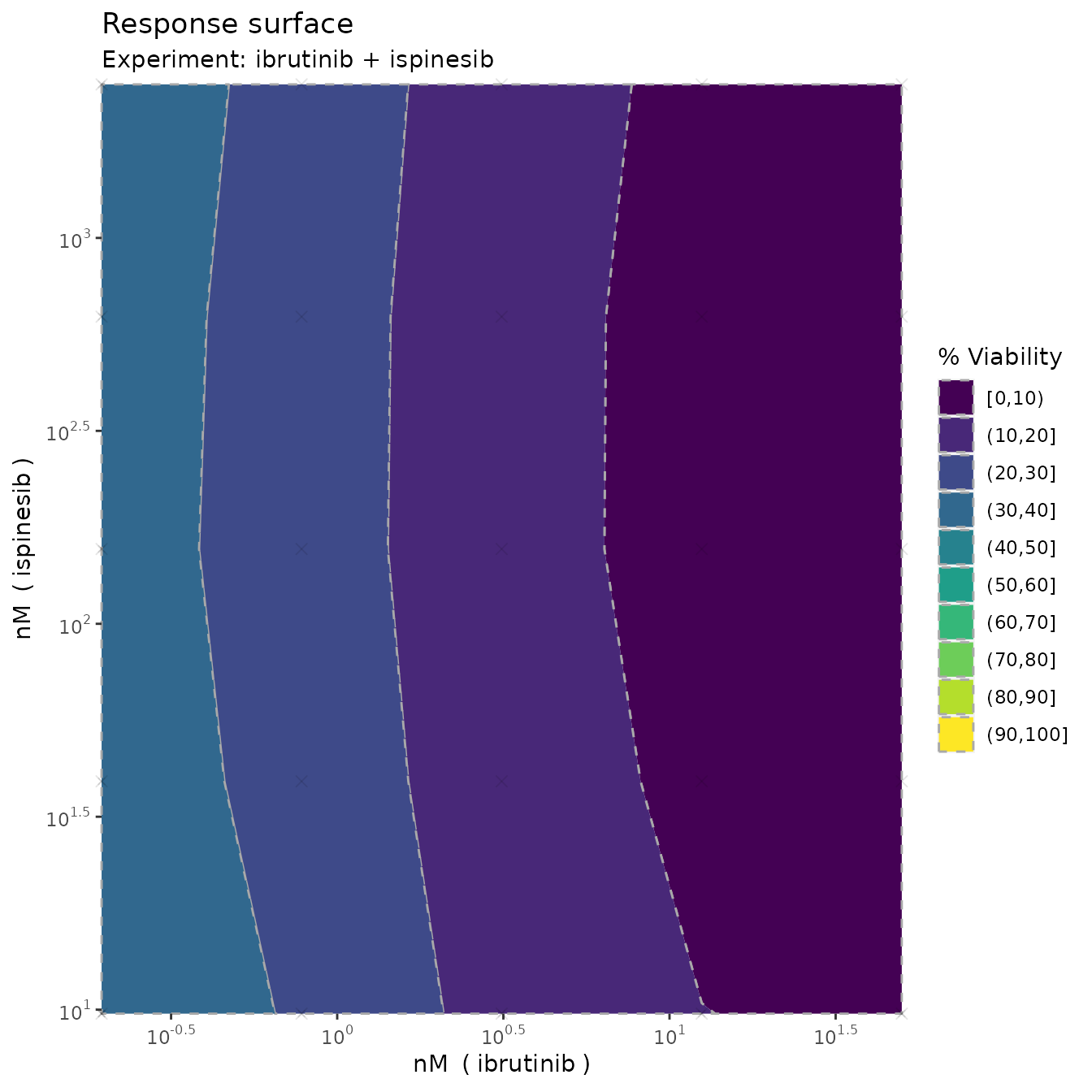
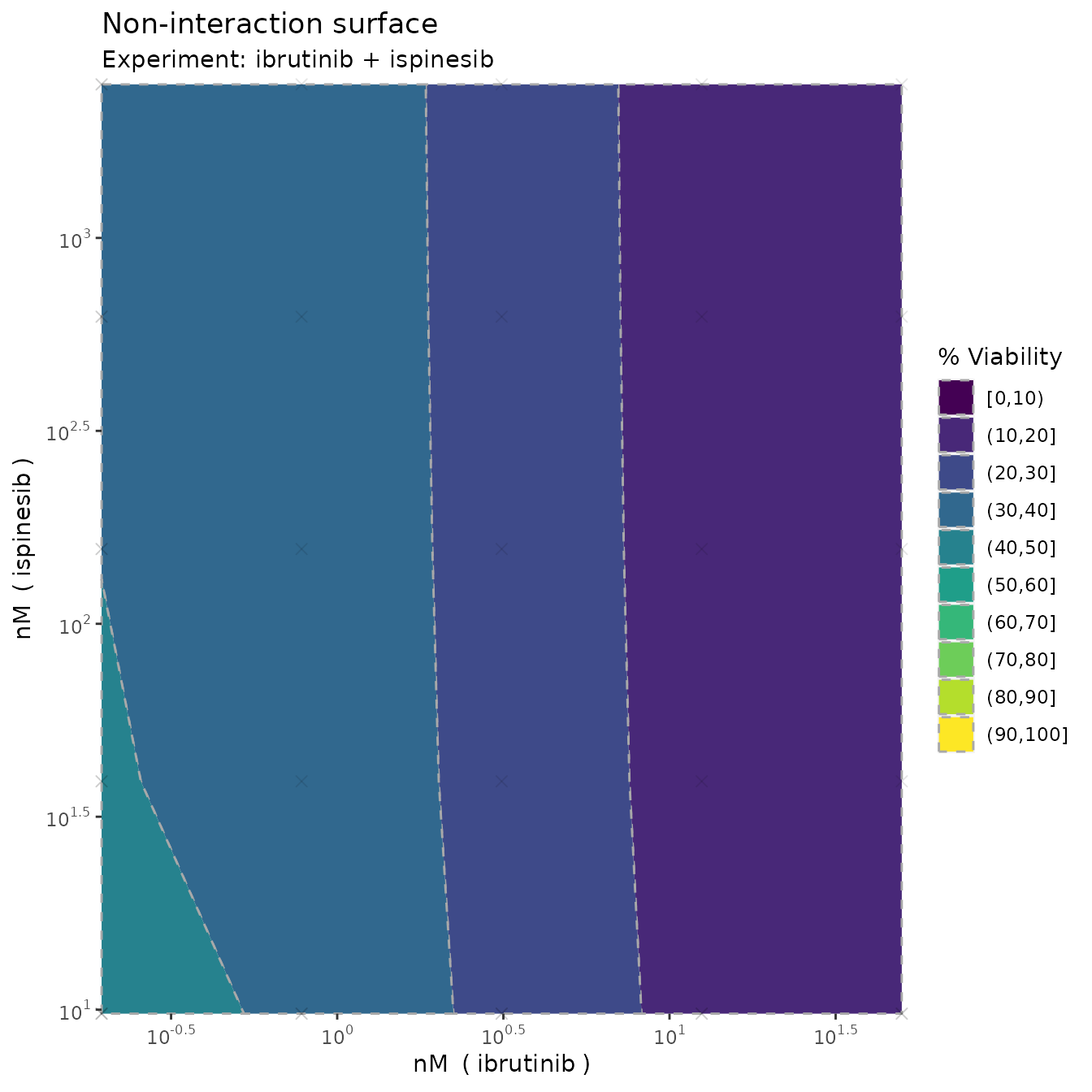
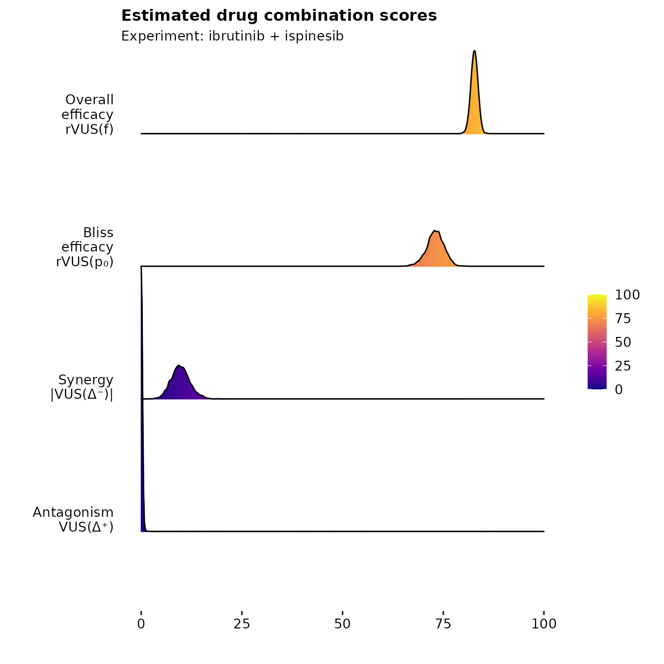
which produces monotherapy curves, monotherapy summary statistics, 2D contour plots of the dose-response function $f$, the non-interaction assumption $p_0$ and the interaction $\Delta$. The last plot displays the $rVUS$ scores as discussed previously, with corresponding uncertainty.

3D interactive plots

The package can also generate 3D interactive plots by setting plot3D = T. These are displayed as following using the plotly library (Plotly Technologies Inc. (2015)).

Dose-response

Non-interaction

Interaction

References

Plotly Technologies Inc. 2015. “Collaborative Data Science.” Montreal, QC: Plotly Technologies Inc. 2015. https://plot.ly.