Introduction to bayesynergy • bayesynergy

The bayesynergy R package implements a Bayesian semi-parametric regression model for estimating the dose-response function of in-vitro drug combination experiments. The Bayesian framework offers full uncertainty quantification of the dose response function and any derived summary statistics, as well as natural handling of replicates and missing data. The Bayesian model is implemented in RStan, taking advantage of the efficient ‘No U-Turn Sampler’ as well as variational Bayes for quick approximations of the true posterior.

The package is further equipped with plotting functions for summarizing a drug response experiment, parallel processing for large drug combination screen, as well as plotting tools for summarizing and comparing these.

Basic usage example

To get started, simply load the package with

library(bayesynergy)

We have included an example dataset from a large drug combination screening experiment on diffuse large B-cell lymphoma. To access it, simply run

data("mathews_DLBCL")
y <- mathews_DLBCL[[1]][[1]]
x <- mathews_DLBCL[[1]][[2]]
head(cbind(y,x))

##      Viability ibrutinib ispinesib
## [1,] 1.2295618    0.0000         0
## [2,] 1.0376006    0.1954         0
## [3,] 1.1813851    0.7812         0
## [4,] 0.5882688    3.1250         0
## [5,] 0.4666700   12.5000         0
## [6,] 0.2869514   50.0000         0

where y contains the measured post-treatment viability, and x the corresponding drug concentrations of the two drugs.

To fit the model, simply run

fit <- bayesynergy(y,x)

and wait for the sampling process to complete.

The results can then be plotted to inspect the model fit e.g. for the monotherapies

plot(fit)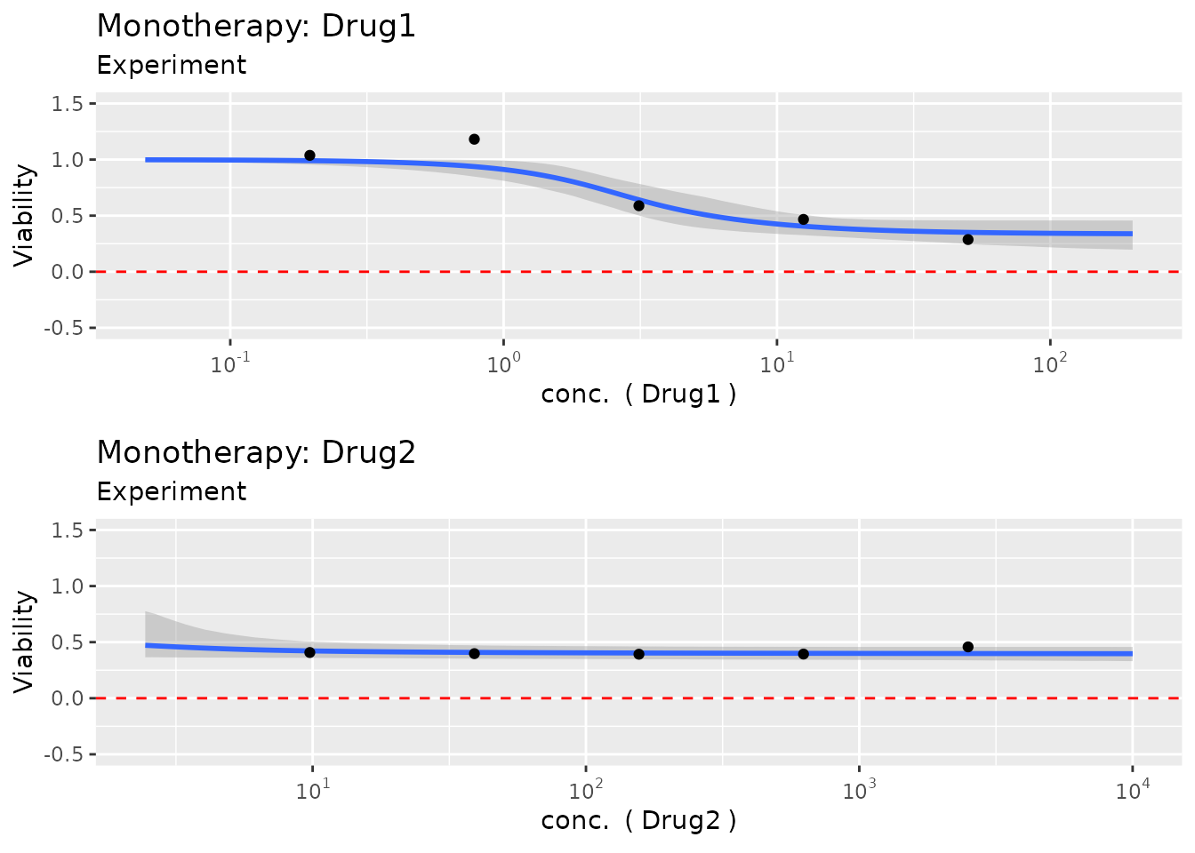

And similarly for the full dose-response surface in an interactive figure

Quantitative measures of drug response and synergy, alongside summaries of the model parameters can be extracted by running

summary(fit)

##                 mean  se_mean     sd      2.5%       50%  97.5% n_eff  Rhat
## la_1[1]       0.3301 0.002757 0.0782  1.29e-01  3.44e-01  0.453   804 1.005
## la_2[1]       0.3866 0.002824 0.0652  1.40e-01  3.97e-01  0.458   533 1.008
## log10_ec50_1  0.4866 0.005445 0.1636  2.48e-01  4.48e-01  0.908   902 1.004
## log10_ec50_2 -1.0332 0.019955 1.0356 -3.41e+00 -8.69e-01  0.491  2693 1.000
## slope_1       2.0305 0.020574 0.9436  8.39e-01  1.82e+00  4.462  2103 1.002
## slope_2       1.4765 0.017784 1.0723  1.05e-01  1.22e+00  4.218  3636 1.001
## ell           3.0663 0.034693 1.5244  1.24e+00  2.71e+00  6.958  1931 1.002
## sigma_f       0.8416 0.017847 0.8069  1.70e-01  6.09e-01  2.830  2044 1.002
## s             0.0969 0.000275 0.0149  7.30e-02  9.52e-02  0.131  2956 1.000
## dss_1        33.5129 0.043268 2.8622  2.76e+01  3.36e+01 39.018  4376 1.000
## dss_2        59.4368 0.042907 2.8725  5.36e+01  5.95e+01 64.731  4482 1.000
## rVUS_f       82.7751 0.013496 0.8629  8.11e+01  8.28e+01 84.453  4088 1.000
## rVUS_p0      73.0558 0.031947 2.2230  6.85e+01  7.31e+01 77.257  4842 0.999
## VUS_Delta    -9.7193 0.034040 2.3820 -1.46e+01 -9.65e+00 -5.295  4897 1.000
## VUS_syn      -9.7633 0.033685 2.3422 -1.46e+01 -9.68e+00 -5.490  4835 1.000
## VUS_ant       0.0440 0.001873 0.1079  5.45e-06  8.02e-05  0.372  3318 1.000
## 
## log-Pseudo Marginal Likelihood (LPML) =  50.9839

For a more detailed look into the functionality of the package, please see the other vignettes.