Predict Top-k Rankings with Pairwise Preferences

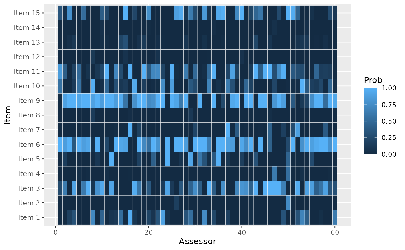
Predict the posterior probability, per item, of being ranked among the top-\(k\) for each assessor. This is useful when the data take the form of pairwise preferences.

Usage

predict_top_k(model_fit, k = 3)

Arguments

model_fit

An object of type BayesMallows, returned from compute_mallows().

k

Integer specifying the k in top-\(k\).

Value

A dataframe with columns assessor, item, and prob, where each row states the probability that the given assessor rates the given item among top-\(k\).

See also

Other posterior quantities: assign_cluster(), compute_consensus(), compute_posterior_intervals(), get_acceptance_ratios(), heat_plot(), plot.BayesMallows(), plot.SMCMallows(), plot_elbow(), plot_top_k(), print.BayesMallows()

Examples

set.seed(1)
# We use the example dataset with beach preferences. Se the documentation to
# compute_mallows for how to assess the convergence of the algorithm
# We need to save the augmented data, so setting this option to TRUE
model_fit <- compute_mallows(
  data = setup_rank_data(preferences = beach_preferences),
  compute_options = set_compute_options(
    nmc = 1000, burnin = 500, save_aug = TRUE))
# By default, the probability of being top-3 is plotted
# The default plot gives the probability for each assessor
plot_top_k(model_fit)

# We can also plot the probability of being top-5, for each item
plot_top_k(model_fit, k = 5)

# We get the underlying numbers with predict_top_k
probs <- predict_top_k(model_fit)
# To find all items ranked top-3 by assessors 1-3 with probability more than 80 %,
# we do
subset(probs, assessor %in% 1:3 & prob > 0.8)
#>     assessor    item  prob
#> 301        1  Item 6 1.000
#> 302        2  Item 6 0.866
#> 303        3  Item 6 0.998
#> 482        2  Item 9 0.892
#> 483        3  Item 9 1.000
#> 601        1 Item 11 0.854

# We can also plot for clusters
model_fit <- compute_mallows(
  data = setup_rank_data(preferences = beach_preferences),
  model_options = set_model_options(n_clusters = 3),
  compute_options = set_compute_options(
    nmc = 1000, burnin = 500, save_aug = TRUE)
  )
# The modal ranking in general differs between clusters, but the plot still
# represents the posterior distribution of each user's augmented rankings.
plot_top_k(model_fit)